

Reference Publication: Parker, D., Fairey, P., McCluney, R., Gueymard, C., Stedman, T., McIlvaine, J., "Rebuilding For Efficiency: Improving the Energy Use of Reconstructed Residences in South Florida", Prepared for U.S. Department of Energy, Florida Energy Office, and Florida Power & Light Company, FSEC-CR-562-92, December 1992. Disclaimer: The views and opinions expressed in this article are solely those of the authors and are not intended to represent the views and opinions of the Florida Solar Energy Center. |
REBUILDING
FOR EFFICIENCY:
Improving the Energy Use of Reconstructed
Residences in South Florida
Danny
Parker, Philip Fairey, Ross McCluney,
Chris Gueymard, Ted Stedman, and Janet McIlvaine
Florida
Solar Energy Center (FSEC)
FSEC-CR-562-92
Executive Summary
On August 24th, 1992, Hurricane Andrew devastated a large part of South Dade County in Florida. With over 35,000 homes to be rebuilt, there is interest in seeing if these reconstructed residences can be made more energy-efficient.
This report provides a comprehensive assessment of potential energy efficiency improvements for both new and existing homes in South Florida. Over forty energy-efficiency measures were considered in the analysis. Many homes in the effected zone experienced damage to their windows, roofs and the surrounding landscape. As a result, the analysis closely examined options associated with these design aspects. All major end-uses of electricity were considered: space cooling and heating, water heating, refrigeration, lighting and other appliances.
Our research considered both the technical feasibility of available methods to save energy as well as the economics of the various options that are available. Optimization analysis was used to choose superior combinations of energy-efficiency measures that will provide maximum energy savings at the lowest possible cost. The study used a combination of monitoring studies and simulation analysis to determine the effectiveness of the various measures.
Results of the analysis showed that while it was technically feasible to reduce household electricity use in South Florida homes by 73 - 84%, the economically cost-effective savings ranged from 39% - 48 %. A group of economically superior measures were identified during the course of the analysis. These included the following improvements beyond the current energy code:
Envelope:
-
Reflective roof or attic radiant barrier
-
Reflective east and west windows or reflective window film
-
White colored walls
Heating and Cooling System:
-
Sealed duct air distribution system
-
Duct system within the conditioned space or reflective roof
-
Air conditioner SEER > 12.0 Btu/W
-
Proper air conditioner sizing
Water Heating:
-
Low-flow showerheads
-
Improved tank insulation
-
Low-cost add-on solar water heater
Appliances:
-
Most efficient refrigerator for size and type
-
Compact fluorescent lighting
-
Halogen incandescent lighting
-
Down-sized pool pump on timer with large piping and filter
The identified package of measures for new construction was estimated to potentially reduce annual electricity consumption in rebuilt homes by 39% or 5,350 kWh at an initial cost of about $3,000. Summer utility coincident peak loads were predicted to drop by 1.5 kW-- about 37% lower than conventional new homes. Annual savings were calculated at approximately $430 with a seven year payback. The after-tax rate-of-return from this level of savings is very favorable at 14% in real terms. The package was estimated to save utility electrical generation at a cost of less than half that of current retail residential electricity prices. Savings for existing homes were predicted to be even higher (7,100 annual kWh), mainly due to the large potential improvements available from improving existing air conditioner efficiencies.
Regardless of the large magnitude of the identified savings potential, our analysis finds that there is still considerable uncertainty associated with a number of the analyzed measures. The study concludes that the certainty of the estimates and the composition of the savings packages may be considerably improved with a well-designed experimental study. We propose a research project with approximately 400 homes (200 control, 200 experimental) for the South Florida area. It is recommended that such a pilot demonstration project be undertaken at the earliest opportunity.
Appendices:
Appendix A: Monitored Residential
Building Energy Use in Florida
Appendix B: Analysis of Energy Losses
of Thermal Distribution System
Appendix C: Collected Cost Data for
Analysis
Appendix D: Window Selection Guidelines
for South Florida Residences
Appendix E: Reflective Roof Research
at FSEC
Appendix F: Appliance and Internal
Load Profiles
Appendix G: Economic Criteria for Analysis
Appendix H: Sample DOE
2.1D Input and Output for Analysis (pdf)
1. Introduction
On August 24th, 1992, Hurricane Andrew exacted tremendous physical devastation on the South Florida area. With top wind gusts of nearly 170 mph the class four storm was one of the most destructive hurricanes of the century. Cutting a 25-mile wide path of destruction across the suburbs of South Miami, at least 85,000 buildings in the area were severely damaged. Estimates show that some 34,000 homes will have to be replaced (WWR, 1992). Many more buildings experienced varying degrees of repairable damage. Many of the structures were single family residences in the communities of Kendall, South Miami, Homestead and Florida City. Over $7 billion in insured losses were sustained (ENR, 1992). Total damages are estimated at approximately $20 billion. Improvements in the code review and inspection process and hurricane resistance of construction methods have justifiably been of the greatest immediate concern (RSI, 1992; Miami Herald, 1992). Implications for structural performance of building materials has been recently covered in a research publication by the American Plywood Association (Keith and Rose, 1992).
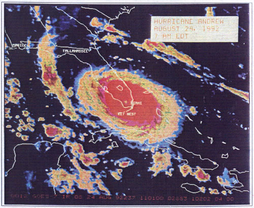
Figure 1: Hurricane Andrew slams into Florida at 7 AM,
August 24th,
photographed by the infra-red camera aboard the GOES-7 satellite.
Color is proportional to atmospheric heat content. The eye of
the
storm is clearly visible over Homestead. (U.S. Weather Service)
However, since the storm, there has been a desire to see if something positive might be accomplished in response to the disaster. Organizations such as We Will Rebuild have already begun an encouraging effort to rejuvenate stricken neighborhoods. One emerging idea is that the new communities might incorporate greater energy efficiency in their reconstruction. In this fashion, the rebuilt homes might become a flagship for energy efficiency potential for residential buildings in the rest of the state.
This study provides a preliminary examination of the various options that are available to improve the energy efficiency of South Florida's residential buildings. Each energy end-use in homes is examined: space cooling and heating, appliances, water heating and amenities. The primary objective is to identify and quantify the savings available from various measures as well as their cost and performance.
The source for the developed information is a combination of monitoring studies, simulation analysis and calculation. A detailed building energy simulation, DOE 2.1D, was used for the analysis of cooling and heating options. Where possible, results were compared to existing field studies to establish the credibility of the results. Measurements and performance data are available for most of the other considered options. Where disputes or differences exist with respect to cost or savings, a range of potentials were examined or conservative assumptions were adopted.
The analysis considered two major building types:
-
New single-family homes that are to be constructed.
-
Existing single-family homes that can be improved.
The analysis calculates savings and performance for all measures relative to a base case. This base is the current Florida building code for new structures, and a typical residential building for existing South Florida homes. All measures were then ranked in terms of their technical potential to reduce energy use. Since interactions between many measures is pronounced, an incremental analysis was also performed to establish the measure specific ranking of the various options. Consideration of costs in the optimization process helps to guide selection of the most cost effective combinations of measures.
2. Residential Energy Use in South Florida
Residential buildings account for roughly half of Florida's electrical energy use and are responsible for approximately $5 billion in annual energy expenditures. As outlined in the current demand side management study (DSM) for the state, FPL's South Florida region accounts for some 23,450 GWh in residential electrical sales (SRC, 1992). This represents greater than one third of all residential electrical energy use in the state. Some 48% of these customers in the area live in single-family homes. The average single-family household in South Florida uses about 15,000 kWh annually.
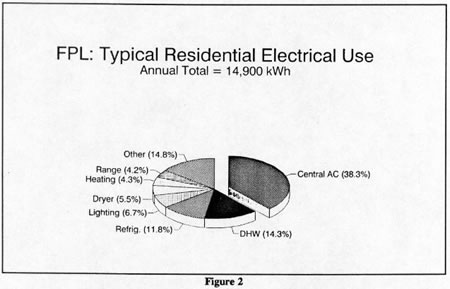
Figure 2 and Table 1 shows the estimated electrical end-uses in a typical Miami home. Also given is the appliance saturation, or percentage of homes possessing various types of electricity using equipment. The energy end uses reflect the hot and humid climate. An estimated 38% of electrical energy is used for air conditioning; space heating is a relatively minor fraction. Refrigeration and water heating both comprise 14% and 12% respectively. The remainder includes lighting, cooking, clothes washing and drying, dish washing and swimming pool pumps. Several appliances are particularly energy-intensive: central air conditioners were estimated to use an average of 5,710 kWh per year, swimming pool pumps use 3,120 kWh, water heaters use 2,130 kWh and freezers and refrigerators use 1,830 and 1,770 kWh respectively.
Typical Electricity End-Use Consumption in South Florida Homes
Typical
End-uses |
Annual
kWh |
Appliances Saturation (%) |
| Central Air Conditioner | 5708 |
78.7 |
| Water Heating | 2134 |
83.3 |
| Frost-free Refrigerator | 1766 |
98.0 |
| Lighting | 1000 |
100.0 |
| Clothes Dryer | 827 |
75.9 |
| Resistance Heating | 644 |
78.0 |
| Range/Oven | 627 |
86.1 |
| Dishwasher | 425* |
66.7 |
| Clothes Washer | 112 |
92.0 |
| Micellaneous | 1669 |
100.0 |
| Total | 14,912 |
---- |
Non-Typical End-uses |
||
| Swimming Pool Pump | 3,117 |
23.6 |
| Heat Pump | 1,309 |
3.9 |
| Room AC | 1,839 |
60.6 |
| Man. Refrigerator | 902 |
8.2 |
| Auto Defrost Freezer | 1,830 |
11.0 |
| Manual Defrost Freezer | 1,321 |
8.2 |
| Source: SRC Energy conservation and Energy Efficiency in Florida: The Second Decade, Phase I Final Report, Synergic Resources Corp., p. C-40, July, 1992. | ||
| * Total for dishwasher energy use includes hot
water use associated with machine operation. Dishwasher energy use itself is < 200 kWh/yr. |
||
The energy demand of Florida homes has important consequences. Each home using the average amount of electricity requires approximately 6 tons of coal, or 160,000 cubic feet of natural gas to produce its annual electricity -- a fact that is becoming more important in Florida as the state is forced to rely more on fossil fuels for meeting its future electrical needs. The combustion of the coal or natural gas will produce between 10 and 18 tons of CO2 annually. Carbon dioxide is the major greenhouse gas which climatologists believe may lead to global warming. This effluent is also not the only concern: for each 15,000 kWh of electricity produced by coal combustion, some 200 pounds of sulfur dioxide are released into the atmosphere -- a major ingredient in the formation of acid rain.
Increases in electrical demand from Florida households leads directly to the need for additional power plants and distribution facilities. Each home added to the utility system an increase in diversified coincident peak demand of approximately 4 kW (Davis and Adams, 1988). Thus, under current efficiencies, each additional 50,000 single family homes will require a 200 MW combined cycle power plant to service them. Of the summer peak demand, over half (2.8 kW) is from central air conditioning systems (FPL, 1988).
Finally, the energy use of South Florida homes has economic implications. At current prices, the average household will spend over $1,200 per year to pay for its electricity use. Given the nearly one million residential customers in single family homes in South Florida, this cost accounts for an energy-related expense of over $1 billion annually to the local economy. These costs are further increased if those living in multi-family or manufactured homes are included in the total.
3. Building Energy Efficiency
A number of means exist with which to reduce energy use in buildings. Since cooling loads comprise the largest portion of overall savings energy use in Florida homes, measures to reduce its magnitude have the greatest overall potential. We first consider an analysis where base existing and new residential buildings are defined. All potential measures are then indexed against these base buildings in order to determine measure-specific savings. However, because of interactions among measures, such individual savings are not additive. This analysis is performed through the use of a detailed building energy simulation.
Improvement Priorities
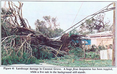
Many of the surviving buildings in the affected area sustained extensive damage. The nature of the damage provides a convenient guide for setting priorities for improvements to South Florida buildings. The vegetative landscape of the region was devastated by the storm. Estimates show that up to 65% of the landscape cover in South Dade was destroyed (Schillaci and Moran, 1992). The 30-mile swath of the maximum storm winds saw the landscape almost totally denuded. The massive loss of trees and shrubs have potentially detrimental impacts on building energy use. Vegetation provides beneficial shading of individual buildings and community level reductions in ambient temperature from shading and evapo-transpiration (Akbari et al., 1992).
Physically, many buildings lost portions of their roofs. With typical construction, the roof portion of the average South Florida home is typically the greatest source of summer heat gain to the structure. Roofing choice, therefore has significant implications for overall energy efficiency. Many homes also lost windows. Window attributes are important in sub-tropical climates since they potentially represent the largest area-normalized cooling loads in residential buildings.
Homes to be totally re-built in the South Florida area offer a potentially greater opportunity for energy efficiency than existing structures. Both frame and block houses can be well insulated and supplied with superior equipment and appliances. Enforcement of the building energy code can provide assurance that the first step in achieving energy efficiency is taken.
Caveats
It is important to note the limitations of this preliminary study. The analysis has been confined to new and existing single family homes. Although, many of the options described here would likely be applicable to multi-family and manufactured homes, no effort has been made to include them in the analysis.
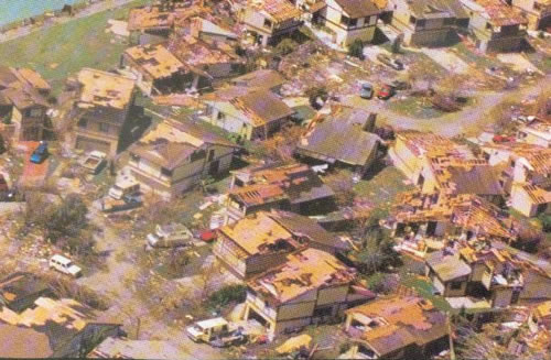
Figure 3: The variety of roofing damaged caused by Andrew
in the Kendall area.
The greatest attention has been paid to performing a sound analysis of the potential savings of the various measures considered. However, actual realized savings will vary in individual cases. Differences in floor area, thermostat schedules, appliance energy use, schedules and ventilation operation can easily vary end-use energy consumption from the average estimates for individual homes by more than 2:1 (Parker, 1990; Lutz, 1992). Also, some measures, such as the shading of air conditioner condensers, do not have well substantiated savings and are impossible to simulate with the current generation software. As a conservatism in such cases, we selected the low end of the savings potential, believing it better to err on the side of savings underestimation.
The most difficult numbers to establish in the study have related to the various measure costs. We attempted to gather several sources on each and to take the mean of the resulting values. This, of course, is subject to the hazards of taking averages on a small sample. Many measures to be considered are not typical practice and therefore have possibly greater current costs than would be reasonably expected with greater market demand and competition.
Although this study recognizes the large potential electricity savings associated with substitution of natural gas for heating, water heating, clothes drying and cooking end-uses, this question has been purposely ignored. Peak load impacts for such substitution can be large, particularly for space heating and cooking end-uses (Shlachtman and Parker, 1981). A more extensive future analysis might do well to consider fuel substitution. However, this should be conducted with an eye to the overall capacity of the existing natural gas pipeline infrastructure and the relative cost/benefit of such measures.
4. Building Simulation Analysis
A detailed hourly building energy simulation, DOE 2.1D, was used to assess methods of reducing the building sensible and latent cooling loads to a practical minimum. DOE 2.1D is a state-of-the-art fourth-generation building energy simulation program that has been developed by the Building Simulation Group at the Lawrence Berkeley Laboratory (LBL, 1984). The program, whose development was sponsored by the U.S. Department of Energy, is a well-documented public domain computer program for analyzing building energy use. DOE-2 predicts the hourly energy use and energy cost of building given hourly weather data, a detailed description of the building, its HVAC equipment and the prevailing utility rate structure. The program is particularly suited to the analysis since over 200 annual simulations were necessary for the analysis. Other simulation models, although some are more detailed, can require several hours of CPU time for a single run. DOE 2.1 performs an annual simulation on a two-zone residential building in about thirty seconds on a VAX 4500.
The simulations were performed on an hourly time step with results compiled, both on an annual basis (8,760 hours) and for the peak summer and winter days. Typical Meteorological Year data (TMY) for Miami, Florida was used for the analysis. The peak summer day was defined as the day in Miami on the TMY tape with the highest cooling loads; the peak winter day was the date with the lowest temperature. These two were August 4th and December 16th, respectively. Current FPL residential utility rates were used for the economic analysis. These rates average $0.08 kWh including fuel-charges and other expenses.
Building Prototypes
A prototype building, representative of residential structures in southern climates, was used for the analysis. The building has a 1,500 ft2 design which is described in detail elsewhere (Fairey et al., 1986). Figure 5 illustrates the building floor plan. Table 2 summarizes the fundamental specifications used for our simulations. The prototypes were created to allow assessment of improvements, both to new building construction, as well as to existing structures:
- Base New Residential Building: This structure represents
current construction practice using typical appliances and established
Florida code levels for thermal integrity. Prototypes were created
for both frame and concrete block construction.
- Base Existing Residential Building: This is a concrete block structure (CBS) reflecting the majority of existing masonry buildings in the damaged area. It contains typical appliances and levels of thermal integrity reflecting the current building stock in the South Florida region.
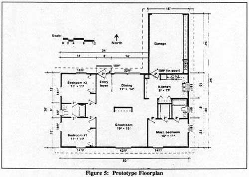
Table 2
Building System Specifications for Base Case Building
| Primary Characteristics | |
| Type: | Single-story, rectangular floor plan |
| Orientation: | Long-axis faces north-south |
| Floor Area: | 1,500 ft²; slab-on-grade |
| Roof: | Asphalt shingles on plywood decking; 22.6º roof slope |
| Overhang: | 2 foot around entire perimeter |
| Ceiling Insulation: | New: R-19 over 1/2" sheetrock Existing: R-11 over 1/2" sheetrock |
| Wall Construction: | New: Frame, R-11 insulation Existing: concrete block, no insulation |
| Wall Absorptance: | 0.6, medium-tan color |
| Roof Absorptance: | 0.8, gray asphalt shingles |
| Windows: | 224 ft²; single glazed with aluminum frame with curtains and some site shading, base shading coefficient = 0.60 |
| Heating and Cooling | |
| Heating: | Resistance strip heat, 30,000 Btu/hr |
| Cooling: | 3-ton AC, SEER = 10.0; SHR = 0.75 |
| Distribution | Attic-mounted duct system; R-4.2 rigid-board fiberglass insulation |
| Appliances | |
| Electric Water Heater: | Storage type, 40 gallon size, 2,134 kWh/yr |
| Existing Refrigerator: | 1,766 kWh per year |
| New Refrigerator: | 1,000 kWh per year |
| Lighting: | Incandescent; 1,000 kWh/yr |
| Clothes Dryer: | 827 kWh |
| Range: | 627 kWh |
| Dishwashers: | 425 kWh |
| Operation | |
| Heating Thermostat: | 70ºF |
| Heating Setback: | 68ºF (8 AM - 5 PM; 12 - 7 AM) |
| Cooling Thermostat: | 78ºF |
| Cooling Setup: | 80ºF (8 AM - 5 PM) |
| Internal Heat Gains: | Averages 648 W |
| Cooling Season: | March - October |
Schedules
We assume three occupants in the prototype home with typical electrical appliances and associated energy use. The specific end-use electrical demand profiles were taken from sub-metered appliance load data gathered from a large sample of homes during the summer months (Pratt et al., 1989). These aggregate profiles were then used to create a schedule for internal heat gains in the building. All simulation inputs were checked against established EPRI guidelines for engineering methods used for such analysis (AEC, 1992).
The thermostat schedule was based on a study by a Florida utility which monitored thermostat settings of a number of residential buildings (Gulf Power Co., 1987). The "base case" building was intended to be representative of conventional residential building practice in the Florida area. From this "reference" building, simulations were performed parametrically to examine the individual effects of each energy efficiency measure (EEM) considered. This allowed identification of the most promising options.
5. Energy-Efficiency Measures
Table 3 summarizes the various EEMs considered in our initial analysis.
Table 3
Listing of the Studied Measures
Measure Title |
Description |
| 1. Base 2. Adv. Heat Pump 3. Hi-Eff. Heat Pump 4. H. Eff. AC 5. Zoned Building 6. Programmable Thermostat 7. Duct System Interior 8. Seal Duct System 9. Radiant Barrier 10. Reflective Roof 11. R-30 Attic Insulation 12.Landscaping (mature) 13. Landscaping (new) 14. Shade AC Condenser 15. Dbl-Pane Low-E, SS 16. Dbl-Pane Low-E, Refl. 17. Dbl-Pane windows 18. Single Pane, Lam/Low-E 19. Single Pane, Reflective 20. Single Pane, SS 21. Single Pane w/ Window Film 22. Single Pane, Refl. E/W 23. Window Awnings 24. R-19 Walls 25. Insulated Door 26. White Walls 27. Whole House Fan 28. Ceiling Fans 29. Infiltration Control 30. Reduce Appliance Gains |
Base Building Advanced heat pump (SEER=15.5; HSPF=10.0) High Eff. H. Pump (SEER=12; HSPF=8.0) High Eff. Air Conditioner (SEER=12.0) 50% of building conditioned: 2 AC systems Programmable thermostat installed Duct system located within conditioned space 70% of duct leakage sealed Attic radiant barrier installed Reflective roof coating applied Attic insulation increased from R-19 to R-30 Mature tree canopy shades 67% of walls/windows Newly installed landscape shades 25% of walls Landscape shading of AC condenser Double pane, low-E spectrally selective windows Double pane, low-E reflective Double pane, aluminum frame, 3/8" air space Single pane, laminated, low-e with selective coating Single pane, reflective coating Single pane, selective surface Reflective window film applied to windows As above but only on east and west windows Fabric or metal window awnings installed Wall insulation increased to R-19 R-5 metal door installed White colored walls Add 36" whole house fan to increase ventilation potential Add 6 ceiling fans to increase ventilation potential Weather stripping and caulking High Eff. Refrigerator and lighting cuts gains |
6. Simulation Results
New Frame Construction
The simulations were completed on an annual basis with each parametric run being compared with the base case. Results are summarized in Table 4 ranked by the measures providing the greatest overall electrical consumption savings relative to the reference configuration:
Table 4
Parametric Simulation Results for New Frame Construction
| Measure Description |
Heating kWh |
Cooling kWh |
Total kWh |
Difference kWh |
Heating Peak kWh |
Cooling Peak kWh |
| Reference Case | 555 |
4788 |
5344 |
0 |
4.03 |
2.43 |
| Advanced Heat Pump | 362 |
3177 |
3538 |
1806 |
1.76 |
1.61 |
| Zoned Building | 365 |
3661 |
4027 |
1317 |
2.51 |
1.70 |
| Dbl. Pane, Low-E, SS | 370 |
3811 |
4181 |
1163 |
2.86 |
2.00 |
| Landscaping (mature) | 702 |
3549 |
4251 |
1092 |
4.11 |
2.01 |
| Dbl. Pane Low-E, Refl. | 418 |
3901 |
4319 |
1025 |
3.12 |
2.04 |
| Duct System Interior | 476 |
3960 |
4436 |
908 |
3.45 |
2.01 |
| Single Pane, Lam. Low-E | 571 |
3873 |
4444 |
900 |
3.75 |
2.09 |
| High Eff. Heat Pump | 392 |
4085 |
4477 |
867 |
1.91 |
2.08 |
| Single Pane, Refl. | 643 |
3970 |
4613 |
731 |
4.08 |
2.15 |
| Hi. Eff. Air Conditioner | 555 |
4087 |
4642 |
701 |
4.03 |
2.08 |
| Sealed Duct System | 511 |
4190 |
4701 |
643 |
3.70 |
2.13 |
| Window Awnings | 628 |
4094 |
4722 |
622 |
4.07 |
2.20 |
| Single Pane, SS | 621 |
4160 |
4780 |
563 |
4.07 |
2.22 |
| Refl. Dbl.: E/W Windows | 519 |
4378 |
4898 |
446 |
3.75 |
2.21 |
| Reflective Roof | 579 |
4335 |
4914 |
430 |
4.04 |
2.21 |
| Landscaping (new) | 597 |
4334 |
4931 |
413 |
4.05 |
2.27 |
| Radiant Barrier | 555 |
4389 |
4944 |
400 |
4.04 |
2.23 |
| Whole House Fan | 555 |
4400 |
4956 |
388 |
4.03 |
2.43 |
| Ceiling Fans | 541 |
4422 |
4963 |
381 |
3.99 |
2.25 |
| Dbl. Pane Windows | 397 |
4593 |
4989 |
355 |
3.24 |
2.30 |
| Single Pane, Refl.: E/W | 587 |
4405 |
4992 |
352 |
4.04 |
2.26 |
| Reduce Appl. Gains | 660 |
4376 |
5037 |
307 |
4.19 |
2.33 |
| R30 Attic Insulation | 468 |
4648 |
5116 |
228 |
3.71 |
2.31 |
| Programmable Thermostat | 511 |
4607 |
5118 |
226 |
4.03 |
2.54 |
| Shade AC Condenser | 555 |
4675 |
5231 |
113 |
4.03 |
2.37 |
| R19 Walls | 474 |
4762 |
5236 |
108 |
3.69 |
2.39 |
| Infiltration Control | 532 |
4721 |
5253 |
91 |
3.89 |
2.38 |
| White Walls | 560 |
4701 |
5261 |
82 |
4.03 |
2.41 |
| Insulated Door | 538 |
4778 |
5315 |
28 |
3.96 |
2.43 |
The simulation analysis results for new South Florida homes showed that all proposed measures would provide some level of energy savings. However, the individual improvements showed varying degrees of effectiveness. The more productive individual measures included high efficiency heat pumps or air conditioners, high performance windows, the shading from mature landscaping and the location of the duct system within the conditioned space of the building. All these options provided stand-alone reductions in annual heating and cooling energy use of 20% or more.
Concrete Block Construction
Recognizing that block construction is a large fraction of new residential buildings in South Florida, we also created a CBS residential prototype. The energy code in Florida requires only a minimum R-3 insulation (1-inch of fiberglass) be installed on the concrete block wall interior. We analyzed measures which we believed would have significant interactions with concrete walls. This included increased insulation, both interior and exterior, changes to wall color and landscape shading. The results are given in Table 5. They show that CBS construction under code levels of thermal integrity are generally equivalent to R-11 frame walls. They also indicate that increases to concrete block wall insulation level on the interior do not significantly improve performance in Miami. However, increased insulation on the exterior of the concrete block walls, does provide reductions in both heating and cooling energy use. We did find that landscape shading of walls was a more important improvement for concrete block than for frame construction. This is due to the lower insulation level.
Table 5
Simulation Results for New CBS Construction
| Measure Description |
Heating kWh |
Cooling kWh |
Total kWh |
Difference kWh |
Heating Peak kWh |
Cooling Peak kWh |
| 1. Frame Case | 555 |
4788 |
5344 |
72 |
2.43 |
4.03 |
| 2. Block Reference Case* | 592 |
4680 |
5272 |
0 |
2.39 |
4.33 |
| 3. Block/R-11 int | 476 |
4733 |
5209 |
-63 |
2.37 |
3.77 |
| 4. Block/R-11 ext | 337 |
4464 |
4801 |
-471 |
2.24 |
3.21 |
| 5. Block/White Walls | 627 |
4530 |
5157 |
-115 |
2.34 |
4.36 |
| 6. Block/Landscaping (new) | 658 |
4209 |
4867 |
-405 |
2.23 |
4.37 |
| 7. Block/Landscaping (mature) | 823 |
3404 |
4227 |
-1045 |
1.97 |
4.45 |
* Light-weight 8" concrete
blocks with R-3 fiberglass insulation on the interior. |
||||||
Analysis of Architectural Influences on Energy
Several parametric runs were performed to the determine the influence of common architectural options. These included the impact of non-optimal building orientation (long axis of the building faces east/west), the benefits of overhangs (the standard building has 2 foot overhangs around the entire perimeter), the energy liability of a 2 x 4 foot south facing single-glazed skylight and the added infiltration from a poorly sealed fireplace (no damper). In the later case, the average infiltration rate (0.4 ACH) was increased by 10%.
Table 6
Simulation Results for Analysis of Architectural Features
| Measure Description |
Heating kWh |
Cooling kWh |
Total kWh |
Difference kWh |
Heating Peak kWh |
Cooling Peak kWh |
| 1. Reference Case | 555 |
4788 |
5344 |
0 |
2.43 |
4.03 |
| 2. East/West Orientation | 555 |
4933 |
5489 |
145 |
2.55 |
4.04 |
| 3. No Overhangs | 555 |
4879 |
5434 |
90 |
2.47 |
4.04 |
| 4. Skylight | 560 |
5013 |
5573 |
230 |
2.52 |
4.08 |
| 5. Fireplace | 574 |
4842 |
5416 |
72 |
2.48 |
4.13 |
| 6. No Natural Ventilation | 555 |
6498 |
7053 |
1709 |
2.43 |
4.03 |
The results verify traditional architectural wisdom. Adequate cross-ventilation to avoid air conditioning during milder weather conditions can make a large difference (32%) in annual space cooling energy use. A north-south orientation reduces space energy use by about 3% relative to an east-west facing. A standard 2 foot overhang reduces energy consumption by about 2%. Skylights and fireplaces are efficiency liabilities.
Existing Homes
Table 7 presents the analysis results for the various measures analyzed for existing South Florida houses. The base case is a typical CBS structure with uninsulated walls and R-11 insulation in the attic. The last two parametric runs in the table examine the increased use associated with no attic insulation and a reflective roof substituted on such buildings that cannot be insulated.
Table 7
Simulation Results for Existing Construction
| Measure Description |
Heating kWh |
Cooling kWh |
Total kWh |
Difference kWh |
Heating Peak kWh |
Cooling Peak kWh |
| Reference Case | 1043 |
6033 |
7076 |
0 |
5.92 |
3.73 |
| Super Eff. Heat Pump | 740 |
3133 |
3873 |
3203 |
3.01 |
1.70 |
| High Eff. Heat Pump | 740 |
4035 |
4775 |
2301 |
3.01 |
2.21 |
| High Eff. A/C | 1043 |
4040 |
5083 |
1993 |
5.29 |
2.21 |
| Mature Landscape | 1443 |
4214 |
5657 |
1418 |
6.29 |
3.09 |
| Awnings | 1279 |
4852 |
6131 |
944 |
6.21 |
3.29 |
| Sealed Duct System | 959 |
5353 |
6312 |
764 |
5.44 |
3.09 |
| Ceiling Fans | 1025 |
5298 |
6323 |
753 |
5.90 |
3.28 |
| Reflective Roof | 1086 |
5359 |
6446 |
630 |
5.94 |
3.40 |
| New Landscape | 1167 |
5358 |
6525 |
551 |
5.97 |
3.48 |
| Whole House Fan | 1043 |
5503 |
6546 |
530 |
5.92 |
3.73 |
| Window Film: E/W | 1062 |
5565 |
6627 |
449 |
5.79 |
3.48 |
| R-30 Attic | 902 |
5757 |
6659 |
417 |
5.46 |
3.52 |
| White Walls | 1130 |
5585 |
6715 |
361 |
5.96 |
3.56 |
| Reduce Appl. Gains | 1180 |
5551 |
6713 |
345 |
6.07 |
3.61 |
| Programmable T-stat | 967 |
5787 |
6755 |
321 |
5.92 |
3.84 |
| R-19 Attic | 971 |
5888 |
6858 |
217 |
5.68 |
3.63 |
| Shade A/C Condenser | 1043 |
5890 |
6933 |
142 |
5.92 |
3.63 |
| Infil. Control | 1022 |
5958 |
6980 |
96 |
5.81 |
3.67 |
| No Attic Insulation | 1482 |
6908 |
8390 |
-1314 |
7.35 |
4.23 |
| No Attic/Refl. Roof | 1602 |
5407 |
7009 |
69 |
7.37 |
3.53 |
The simulation results for existing homes show the large potential benefits available for replacing existing lower efficiency air conditioners with newer high-efficiency models. Also, the lack of wall insulation makes white walls or landscape shading relatively more desirable than with new homes. Application of reflective window films was only analyzed for the east and west building faces in interest of preserving interior daylight and for addressing aesthetic concerns.
7. Detailed Description of the Measures
A variety of proven technologies are available to reduce building energy use. Below, we detail the various analyzed measures. Pertinent FSEC research on many of the described technologies is summarized in Appendix A.
Thermal Distribution System
Most South Florida residences feature central air conditioning with an air distribution system located in the attic space. Previous analysis using a very detailed finite element simulation, FSEC 3.0, has shown that Florida residences with such thermal distribution systems potentially use up to 30% more space cooling energy than would a system with sealed duct work within the unconditioned space (Parker, Fairey and Gu, 1992). These losses include both forced air leakage and heat transfer to the attic mounted duct system. Use of the simulation showed that duct heat transfer increased cooling energy use by approximately 8%. Duct air leakage can lead to highly variable increases in cooling and heating energy use. With a typical area of audited duct leakage, loads were predicted to increase by about 14% relative to a system with 70% of the leakage sealed. The combined effect serves to reduce effective air conditioning cooling efficiency by approximately 21%. Examination of the effects under heating conditions showed a similar magnitude of losses. The 21% reduction in efficiency is conservative since measured results from sealing about 70% of discovered duct leakage alone, saw measured reductions in cooling energy use of 17.2% (Cummings et al., 1991). Other studies of the impact of duct losses on overall HVAC efficiency have concluded even greater impacts. Modera et.al., (1992), Koomey (1991) and Andrews (1992) have all cited average reductions to efficiency of 30% or more.
Unfortunately, DOE 2.1D, as currently configured, has no method of comprehensively incorporating duct system heat gains or air leakage to the thermal distribution system (Huang, 1991). This was accommodated in our simulations by adjustment to the seasonal efficiency of the heating and cooling equipment. The exact multipliers used in our analysis for heating and cooling efficiency were based on annual simulation results using FSEC 3.0 and are detailed in Appendix B.
Orientation and Architecture
The energy savings potential of proper building orientation has been long recognized (Olgyay, 1965). Shading from fixed devices, such as overhangs, are also effective in South Florida (Buffington, Sastry and Black, 1981; McCluney, 1983). As part of our parametric analysis, we examined these influences. This was done by changing the prototype building's orientation from the long axis facing north and south (the optimal orientation) to east and west. The savings of fixed shading was examined by deleting the continuous 2-foot overhangs in the building. Typical of current practice, the windows were assumed to be located at a height of 6.75 feet from grade level.
Natural Ventilation
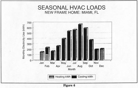
Natural ventilation of residential buildings is an effective and well understood traditional cooling method (Fairey, Chandra and Kerestecioglu, 1986). The base case analysis assumes that South Florida residences are mechanically air conditioned from March 1st through November 30th. This is accomplished by a thermostat setting of 90oF for the non-cooling months. The assumption is that natural ventilation will provide most of the necessary cooling during the three Miami "winter months." Similarly, heating is assumed from December 1st through February 28th. The resulting month-by-month predicted heating and cooling energy use is shown for the new frame base in building Figure 6. We ran a single case where air conditioning was assumed to be used year round. The results of this case allowed a determination of the specific benefit of natural ventilation for reducing air conditioning use. This case, shown in Table 5, indicates that the availability of natural ventilation reduces cooling energy use by 32%, or 1,709 kWh per year over year-round closed building operation.
Whole House Fan
Whole house fans exhaust large quantities of air from the house interior to the attic space. This provides forced ventilation even when local wind velocities are low. Typically fans are operated during the cooler evening hours to take advantage of ventilation rather than air conditioning. Such a strategy provides a longer "ventilation season" in Florida since nighttime windspeeds are typically lowest during the summer months. A recent study in Central Florida found that whole house fans dropped the average nighttime interior temperature by 2 - 6oF when operated during summer conditions (Parker, 1991). This is potentially important since a statistical survey analysis of 384 homes in Central Florida found that each month that a household claimed to use natural ventilation rather than air conditioning averaged annual electricity savings of 388 kWh (Vieira and Parker, 1991).
The implication is that electricity can be saved if the natural ventilation season can be extended and vapor-compression air conditioning is reserved for only the hottest periods. A detailed computer analysis of potential savings from whole-house fans by Kusuda and Bean (1981) for Houston, Texas found a 24% air conditioning savings potential. Burch and Treado (1979) measured the savings of a whole-house fan on air conditioning in a house in Houston. The fan was operated when the temperature outside was less than 82oF and greater than 75oF. They found the air conditioning energy use reduction were well correlated with the daily average outdoor temperature. Savings varied from 65% at 76oF to 10% at 84oF. Of greatest pertinence, however, is a field study of a home in Gainesville, Florida which found a 22% air conditioning savings using a similar control strategy with a whole house fan in the summer of 1982 (Ingley et al., 1983).
Our study made simple and conservative assumptions relative to the potential savings of whole house fans, checking reasonableness of our results against the above field studies. We assumed that whole house ventilation could obviate the need for air conditioning in the months of February - April and October and November in Miami. Based on an electric demand of 300 Watts and 12 hour operation, we assumed 3.6 kWh per day is used by fan operation. The differential between the predicted air conditioning energy consumption for these months and the average 110 kWh for whole house operation comprised realized savings. As expected, savings were greatest for the months of October and April, but were still less than 200 kWh per month.
One consideration which can serve to greatly reduce the effectiveness of this strategy is consideration of humidity levels. Restriction of outdoor air ventilation to periods when the air temperature is between 82o and 75oF exacts one limitation. However, limitation to periods when relative humidity is less than 70% will greatly reduce its effectiveness. We assumed that this was not a limitation, although it does create a bias against general application of this option.
Ceiling Fans
The ability of ceiling fans to improve human comfort during the cooling season is well understood (Fairey, Chandra and Kerestecioglu, 1986). We examined the added cost of installing six quality ceiling fans ($600) and assumed this would allow the cooling thermostat setting to be elevated by 2oF when occupants were home. This increased the cooling thermostat setting to 80oF. The house was assumed to be occupied between 5 PM and 8 AM on weekdays and all day on weekends. The analysis is based on the fans running an average of eight hours per day on medium speed, drawing 30 watts each. This electricity consumption (44 kWh/month) was added to the DOE 2.1D estimated cooling energy use. The building's internal heat gains were also increased by 205 Btu/hour to account for the additional heat released from operation of the fans.
Simulation results showed an 8% reduction in space cooling energy use for new homes even after the direct energy use of the ceiling fans and internally released heat was taken into account. Savings were over 12% for existing homes. However, it must be pointed out, that the realized savings of this measure is exceedingly sensitive to thermostat behavior in response to fan use (see Figure 4 and associated discussion).
Heating and Cooling Equipment
The relative efficiency of heating and cooling equipment in residences has a direct impact on building energy use. The long cooling season in Miami suggests the importance of air conditioning equipment efficiency and capacity. Several field studies exist showing excellent savings from the substitution of high efficiency air conditioning equipment in replacement of existing less efficient units (Parker, 1990; Burns and Hough, 1991; Ternes and Levins, 1992). Measured savings were on the order of 20 - 40% of pre-retrofit cooling consumption.
We assume that the Seasonal Energy Efficiency Ratio (SEER) of existing Miami residential air conditioning equipment averages 8.0 Btu/W. The equipment has an average 36,000 Btu/hr (3-tons) capacity with a sensible heat ratio of 0.75. Typical new air conditioning equipment is assumed to consist of a three-ton SEER 10.0 air conditioner. Both new and existing buildings are assumed to have strip heat (forced air resistance heating systems).
High efficiency air conditioners are assumed to be SEER 12.0 with an incremental cost over standard units (SEER 10) of approximately $400 (Cummings, 1988). Similarly, the high-efficiency heat pump has an SEER of 12.0 with a Heating Season Performance Factor (HSPF) of 8.0 Btu/W. This option has an incremental cost of $1,200 relative to a straight SEER 10.0 air conditioning system.
An advanced heat pump is also analyzed, representing the most efficient air-to-air equipment currently available. It is based on an variable-speed Carrier unit with an SEER of 15.5 and a HSPF of 10.0.
This configuration has an incremental cost of approximately $2,500 relative to a straight three-ton SEER 10.0 air conditioner. The validity of the above cost data was established through a series of contacts with local air conditioning and heating contractors (see Appendix C).
Our analysis indicated this to be one of the most effective efficiency improvement options. The advanced heat pump demonstrated the potential of reducing energy use by 33% in new construction and by 45% in existing buildings. Both heating and cooling peak loads were also substantially reduced. Note, however, that the DOE 2.1 predicted reductions to peak cooling loads are likely misleading for variable-speed air conditioning units since they may have higher demand under full load than conventional single-speed high-efficiency units (Henderson, 1990).
Programmable Thermostat
One potential measure is a fully programmable thermostat to control the heating and cooling system. These thermostats allow seven-day scheduling of temperature control including holidays. The primary advantage is that of reliably setting back or up the thermostat when the building is unoccupied. We conservatively assume that the impact of the programmable thermostat will be to increase the depth of the setback or setup by 1oF. The justification is that the increased setback/setup will be realized due to the improved reliability with which the changed settings are made. The normal heating season setback is 68oF from 11 PM to 7 AM and from 9 AM to 5 PM during weekdays. The normal cooling season setup is 80oF from 9 AM to 5 PM during weekdays. There is no setback or setup during daytime hours on weekends or holidays. Programmable thermostats cost between $70 and $150. We assume the measure costs $200 including installation.
Simulation results showed that the option reduced heating and cooling energy use by about 4% for new buildings, although actual savings would be very sensitive to the degree of setback or setup achieved in individual cases. We also, note that this strategy has the potential of aggravating peak loads, since the heating or cooling system is often activated during periods coincident with utility system peak loads.
Zoning
Air conditioning contractors have long known that zoning the sections of a home so that only part of the space is conditioned can save electricity. Analysis of potential energy savings from zoning was accomplished as follows: The 30 x 50 foot rectangular living space in the prototype was sectioned into two separate 30 x 25 foot zones separated by an uninsulated partition wall and a closed door. One section of the home was then conditioned for the evening hours from 11 PM to 7 AM; the other section was conditioned for the remainder of each day.
The thermostat schedule was apportioned and internal heat gains were split between the two spaces. Rather than a single 3-ton air conditioner; we assumed that a separate two-ton AC was used for each space along with required duct work and separate thermostatic controls. The cost premium for the two air conditioners and added detail for the distribution system and thermostats was determined to have an incremental cost of $1,200.
As expected, analysis showed this to be a very effective strategy to reduce heating and cooling energy use. However, we did not include it in the incremental savings analysis or in the overall economic assessment. This was not done because the measure involves a reduction in amenity for the household, and we desired that our final analysis be life-style neutral for its prime recommendations. For those who do not find such partitioning objectionable, the strategy can provide considerable savings. Estimates indicated a 25% reduction in combined heating and cooling energy use.
Window Options and Shading
A variety of window types were simulated for the new building prototype. A much more detailed description of the different products and their characteristics is contained in Appendix D and a simultaneously issued FSEC research report (McCluney and Gueymard, 1992). Table 8 summarizes the input data used for the simulated glazings. All windows were assumed to be installed in thermally-broken aluminum frames. The U-values for various glazings were modified according to the frame types in Table 13 of Chapter 27 of the Handbook of Fundamentals (ASHRAE, 1989). Double-pane windows were assumed to be separated by a 3/8" air space.
For existing buildings, the analysis was confined to the base case (single pane, clear) and single pane with reflective window film added as the retrofit measure. Based on a previous analysis (Parker, 1989) we examined window treatments to east and west windows as a competing measure with uniform changes to all windows. The greater solar exposure of these building faces provide superior thermal and economic performance. This was also based on a desire to address concern for aesthetics (the most effective films are reflective) and to prevent daylight levels on the interior from being excessively reduced. "Dark windows" which reduce interior levels of illumination and lead to increased use of artificial lighting can nullify any potential thermal savings.
Table 8
Simulated Window Characteristics
Code |
Description |
Shading Coefficient |
U-Value (Btu/hft²ºF) |
Visible Transmittance |
Incremental $ Cost/ft²* |
| SP | Single-pane glass, clear | 1.00 |
1.10 |
90% |
$0.00 |
| SPR | Single-pane, reflective coating | 0.51 |
1.10 |
27% |
$2.00 |
| SPWF | Single-pane/reflective window film | 0.42 |
0.79 |
50% |
$3.00 |
| SPSS | Single-pane with selective surface (blue) | 0.62 |
1.10 |
72% |
$4.30 |
| SPLAM | Single-pane/laminated with low-e film | 0.39 |
0.87 |
54% |
$10.00 |
| DP | Double-pane, 3/8" airspace | 0.81 |
0.60 |
82% |
$2.50 |
| DPLESS | As above with selective surface | 0.33 |
0.37 |
56% |
$10.00 |
| DPR | Double-pane with reflective film | 0.42 |
0.60 |
26% |
$6.00 |
* Includes frame and installation. |
|||||
Our analysis assumed that pre-existing window shading was present in the form of curtains, blinds, landscaping and shadowing from adjacent buildings. All these factors were estimated to change the base case shading coefficient from single-pane clear glass from 1.0 to 0.6. This more realistic assumption tends to reduce the magnitude of the savings realized from window shading and glazing changes. The characteristics for individual glazing systems were then used to modify the shading coefficient input into the model. Similarly, we used the Handbook of Fundamentals to determine an average shading coefficient for awnings. Cost data was collected from vendors of the various glazing types and shading devices. As expected, many of the higher performance glazing types have premium prices.
Analysis results showed high performance windows to be among the most promising measures in terms of energy savings for new buildings. "Superwindows" with low-e coating, a selective surface and a high visible transmittance demonstrated the potential of reducing space conditioning loads by up to 22% in new residential buildings. As expected, savings were disproportionately greater for adding high performance windows to the east and west faces of the analyzed buildings.
Landscaping
With sustained winds exceeding 140 mph, Hurricane Andrew destroyed or damaged the majority of the trees in South Dade County. Re-establishing the landscape can help to save energy. The energy savings potential for landscaping in South Florida has been well established by experimental studies performed at Florida International University (Parker, 1983). Recognizing the changing potential of this measure over the building life, we estimated savings of both newly installed vegetation and of a mature landscape with fully grown tree canopies. In either case, the landscape planting is to be strategically placed to provide shade to the east, west, southeast, and southwest faces of the prototype building. We assumed that the newly installed landscape would shade 25% of the walls and windows in these directions; the mature landscape was assumed to provide 67% shading. As a conservatism, no credit was taken for possible temperature reductions due to evapo-transpiration. The shading is provided from the purchase of six 6 - 8 foot live oak trees. The installed purchase price of these specimens, with a six-month guarantee, was $740. Several nurseries provided similar price estimates.
A recent EPA study recommends shading of exterior air conditioning condensers, using landscaping or other means, as a method to reduce space cooling energy use (Akbari, et.al., 1992). Estimated theoretical savings of such a strategy have ranged from 1 - 10% (Parker, 1983; Abrams, 1986). Unfortunately, no empirical research has been conducted to measure the actual cooling energy savings that can be achieved with this strategy. Given the uncertainty, we chose a conservative estimate with the AC condenser shading conferring a 2% enhancement to the air conditioner seasonal efficiency. This assumes the air temperature being drawn into the condenser unit is dropped by about 2oF by the cooling influence of the landscaping. The benefits are provided by two 6 - 8 foot live oak trees which are located near the condenser unit if it is on the east or west faces of the home. Alternately, location of the condenser on the north face of the home could provide the shading benefits at virtually no cost.
Simulation results showed that a newly installed strategically planted landscape would be able to reduce cooling energy use by about 10%. A mature landscape with shading of the AC condenser could result in a reduction of up to 28%.
Attic/Ceiling Measures
Attic thermal performance is critical in cooling dominated climates since it affects heat gain across the ceiling surface. Control of attic temperatures is doubly important if air distribution ducts are located within this space, as is common in Florida home construction.
Radiant Barriers
A radiant barrier system (RBS) is a layer of low-emissivity foil material placed in an attic airspace to block radiant heat transfer between the hot roof and the top of the ceiling insulation. Extensive research at FSEC has proven that roof mounted RBS can reduce ceiling heat flux by 30 - 50% with annual cooling electricity savings of 7 - 12% (Fairey et al., 1986, 1988, 1989; Ober, 1991). Reductions to peak cooling loads are generally higher. Appendix A includes a comparison of the air conditioning load of two unoccupied frame houses in Gainesville, Florida which were monitored side-by-side with and without a radiant barrier. The RBS was found to save approximately 8% of cooling energy use. Mirroring such measurements, our simulation results predicted an 8% reduction in space cooling energy associated with the installation of a RBS.
A radiant barrier was estimated to cost $325 installed in the prototype building. Cost data were estimated through contacts with several vendors (see Appendix C). The range is in general agreement with the costs encountered in a recent residential retrofit program in Oklahoma (Ternes and Levins, 1992). We did not specifically analyze radiant barriers for existing buildings. However, this will be feasible in some South Florida residences with enough attic space, or those which lost their roofs and are having them replaced. The cost/benefit of this measure for existing homes should mirror that for new buildings.
Reflective Roofs
Recent research at FSEC has focused on the influence of roof materials on thermal performance. Six small roof models have been constructed to evaluate the resistance to heat gain of various types and colors of roofing (Chandra and Moalla, 1992). Initial findings are summarized in the paper in Appendix A. Test cases have included black asphalt shingles, a white asphalt shingle roof with a reflective elastomeric coating and a series of red tile configurations. Results show that roof sections with white reflective coatings exhibit superior thermal performance to conventional roofing systems. Similar experimentation has been performed at Oak Ridge National Laboratories (Anderson et al., 1991) which found that reflective coatings significantly reduce the heat flux through roofs and hence building cooling loads. Recent research conducted this summer at FSEC examined the impact of a reflective coating applied to a residence at mid-summer. Air conditioning was monitored for three weeks before and after the coating was applied. Weather normalized air conditioning savings were approximately 20% with a constant thermostat setting and no change in other conditions. Although the attic floor is insulated with six inches of blown fiberglass (~R19), infrared thermography showed significant changes in ceiling heat flux. A synopsis of this research is contained in Appendix E.
Our simulation analysis predicted a 9% reduction in space cooling energy for new buildings with a reflective roof. As expected, estimated savings increase with lower ceiling insulation levels. Existing CBS residences with R-11 attic insulation were predicted to save 11%.
Reflective roofs have other non-house specific advantages over competing roofing options since increasing the community-wide albedo of roofs should serve to reduce the neighborhood air temperature (Bretz et. al. 1992). EPA has recommended increasing the use of white surfaces in hot climates option to reduce the magnitude of the urban heat island (Akbari et al., 1992). Although currently more expensive than radiant barriers and with a shorter measure life, this "community cooling" advantage of reflective roofs is one that radiant barriers and increased attic insulation do not possess.
Our simulation analysis assumed a reflective roof coating could be applied such that the effective roof solar absorptance dropped from 0.80 with gray asphalt shingles to 0.25 with a white roof (DSET Laboratories, 1992). The cost of the roof coating depends on the circumstance of the installation. For new roofs, we base our cost ($600) on the cost of sprayed-on acrylic latex paint. This material can provide the same thermal benefits without the added cost of the elastomer which would not be needed for a new roof. For existing residences, we assume no cost on the premise that the coating is applied as the existing roof is nearing the end of its useful life which increases its longevity while providing the thermal benefits. Since, the coating will significantly increase the life of the existing roofing system, not all costs of the coating should be attributed to its energy savings capability.
Other factors affect the potential for this measure. Since this EEM is in its infancy, we expect that the cost of a reflective roof could come down significantly as products, such as reflective shingles, are introduced (Jones, 1992). We assume a useful life of the measure of only ten years, although many manufacturers claim a greater longevity. Potential problems with mold and mildew staining make this a reasonable conservatism. Obviously, the development of reflective shingles or the use of a white tiled roof or white sheet metal roof would be expected to greatly extend measure life.
The use of reflective roof coatings is particularly attractive for existing homes in South Florida in which the ceiling cannot be insulated. Some of these structures have flat roofs or configurations with little or no accessible attic space. Reflective coatings can offer greatly reduced air conditioning consumption in these homes which were analyzed separately as special case. Results showed a 28% reduction in space cooling energy in existing uninsulated CBS structures, although space heating budgets were somewhat increased.
Attic Insulation
Addition of attic insulation represents a commonly considered energy savings measure for residences. Code levels in new South Florida homes is R-19 which forms our base case. Existing homes are considered to already have R-11 over the ceiling. However, there are still a significant number of residences in Dade County which are uninsulated. Many of these cannot be feasibly retrofit due to physical limitations. These include flat roofed buildings built in the late 1950s and others where there is virtually no cavity between the roof and ceiling.
Ceiling insulation is a well documented method to reduce the rate of heat transfer from the roof to the interior of residential buildings. Field measurement of the retrofit of ceiling insulation from R-11 to R-30 in a test home in Tennessee showed a 16% drop in measured cooling energy use (Levins and Karnitz, 1987). Addition of a radiant barrier system (RBS) in these tests also showed a similar level of cooling energy savings to that of R-30 insulation. However, these measurements were made in a home in which the air distribution system was located in the crawlspace. Larger savings from the RBS would be expected where the ducts were located in the attic, as is common in Florida homes.
We analyzed the impact of increasing attic insulation in existing homes from none at all to R-19; from R-11 to R-19 and from R-11 to R-30. In new homes, we examined the impact of increasing the insulation level from R-19 to R-30. Predicted savings were modest at 4% of overall heating and cooling energy use. Insulation from R-11 to R-30 in existing residences showed a 6% savings.
The incremental costs of these insulation levels are based on collected cost data (Appendix C and Cummings, 1988). It was assumed that the cost of going from R-19 to R-30 was $210; the cost from R-11 to R-19 was $110. Addition of R-19 insulation to an uninsulated ceiling was based on the costs of blown-in fiberglass with an average cost of $200 for the application. The measure was assumed to have a useful life of thirty years.
Reductions to Internal Gains
Reductions to appliance electricity use in Florida homes can be expected to have significant interaction with cooling and heating energy use. The reduced electrical consumption lowers the level of internally generated heat within the structure. This serves to decrease space cooling demand, while increasing heating energy use. However, the effects are not offsetting since heating and cooling efficiencies are usually different. Also, the length of the cooling season is much longer in South Florida.
The internal gain schedule in the analysis is based on measured appliance use profiles detailed in Appendix F. It averages 648 Watts within the conditioned space with a maximum heat gain rate of 1,261 W at 8 PM. Internal heat gains can be reduced by choosing a more efficient refrigerator, compact fluorescent lighting and locating the hot water tank, clothes washer, clothes dryer and freezer outside the conditioned interior. We estimate the combined reduction of these measures to the internal heat gain rate to be approximately 30%. The cost of this measure is difficult to estimate since the major reason for the change out to a more efficient refrigerator or high efficiency lighting is primarily attributable to the direct energy savings of these measures. As a conservatism, however, we assume that one third of the cost is due to the objective of reducing waste heat in the building's interior. For the more efficient refrigerator and lighting this comes to approximately $125.
As expected simulation analysis showed this measure to decrease cooling energy use (-9%) while increasing space heating energy use (+19%). In absolute terms, however, overall space conditioning energy use dropped by 307 kWh or 6% of annual consumption. Obviously, this option will appear more effective when analyzed in a home with a higher heating system efficiency such as a heat pump.
Infiltration Control
Conservative estimates were made for the energy related savings of infiltration control. We assume that caulking, weatherstripping and attention to window and door seals and ceiling and wall penetrations can reduce the building infiltration rate from 0.40 air changes per hour (ACH) by 10% to 0.36 ACH. The small level of reduction is due to the low level of natural driving forces for infiltration in the Florida climate. Although Florida homes are generally leaky, relative to those in more northerly climates, previous studies of wind and thermal buoyancy induced air infiltration in using SF6 tracer gas dilution have found air change rates commonly in the range of 0.1 to 0.3 ACH (Cummings et al., 1991).
The higher air change assumed in the simulations (0.4 ACH) is due to the operation of the air handler in terms of duct leakage and differential pressures within rooms. These are forces that are not as affected by envelope sealing methods. Greater levels of air tightness were not deemed appropriate since this could result in an unacceptably low ventilation rate. This could have serious implications for indoor air quality. The measure was assumed to have a cost of $200, mainly for labor associated with the increased attention to sealing detail with caulking and weatherstripping (Cummings, et. al., 1989). Our simulation analysis showed modest savings (2%) for heating and cooling associated with this measure. Results were similar for existing and new housing.
Wall Insulation and Color
The influence of wall insulation and color on space heating and cooling consumption was modeled as follows: For new buildings, the assumed insulation levels were R-3 on the interior for concrete block and R-11 for frame walls with 2 x 4" studs 16 inches on center. The analysis for existing homes assumes no insulation and concrete block walls. The base case building, both for existing and new structures was assumed to be a light tan color with an effective solar absorptance of 0.6. White walls were assumed to have an effective solar absorptance of 0.3. Parametric runs were performed for both concrete block and frame walls for new construction. Insulation improvements for new housing consisted of R-19 insulation for frame walls with 2 x 6" studs, 24-inches on center. New CBS homes had R-11 insulation on the interior or exterior analyzed as potential improvements. No incremental cost was assumed for painting the walls white versus other colors. Cost for the various insulation improvements are taken from Cummings (1988). Values were checked against cost data assembled in Appendix C.
Simulation analysis results showed a similar magnitude for the annual heating and cooling energy savings for white walls vs. increased wall insulation for new construction (2%). Savings for white walls was greater for uninsulated existing CBS structures (5%).
Concrete Block Construction
A concrete block prototype was created for analysis of new CBS housing. Eight-inch concrete blocks were assumed with a stucco finish and R-3 insulation on the interior with 1/2" sheetrock facing inside. We also examined the addition of R-11 insulation to the interior and exterior. Externally insulated masonry wall construction can provide an inherent thermal storage capability. Both simulation models and empirical research suggest that such exterior insulation schemes will result in lower thermal loads (Fairey et al., 1986, Al-Mofeez and Woods, 1991; Ternes, 1992). Other measures, such as landscape shading and wall color were examined for the block construction case to determine specific differences in influence. The impact of white walls was performed by assuming the white paint with an absorptance of 0.3 was used. Landscape shading assumed that 25% of the walls would be shaded from a newly installed landscape; 67% would be shaded with full tree canopies.
Simulation analysis showed a modest energy reduction associated with R-11 interior insulation (3%), where as exterior R-11 wall insulation was found to be quite effective (10% reduction in heating and cooling loads). White exterior walls provided a 3% reduction in overall heating and cooling loads.
8. Potential Limitations to Realized Savings
A number of considerations may undermine the potential savings available from the described measures for the reconstruction effort. Obviously, lack of concern and apathy towards the overall objective of reducing energy use in the reconstruction is a fundamental obstacle. Many of those rebuilding may not elect to participate in such a program. However, even for well intentioned participants, other factors may exact limitations on realized savings.
Often when energy-efficiency programs do not deliver the expected level of savings, life-style effects are blamed for the shortfall (Davis and Adams, 1988). "Take-back," "snap-back" and "rebound" are all terms that refer to the tendency for consumers to adjust over time to perceived changes in the cost of energy services generated by improvements in energy efficiency. These changes are also known by the micro-economic description of "temporary price elasticity." For example, energy savings due to an air conditioning efficiency program could induce customers to reduce their thermostat setting to increase comfort to a level that they could not previously afford. This diminishes the potential energy savings of the measure. The reality of this fact was observed in a Florida utility study of energy efficient homes, which found the measured summertime thermostat setting of the efficient houses to be 2 - 3oF cooler than the group of conventional residences (Gulf Power Company, 1987). However, "take-back" can also be expressed in other ways, such as more use of air conditioning rather than natural ventilation, increased use of hot water, increased hours of outdoor lighting and so on. Unfortunately, the magnitude of this phenomenon remains poorly researched.
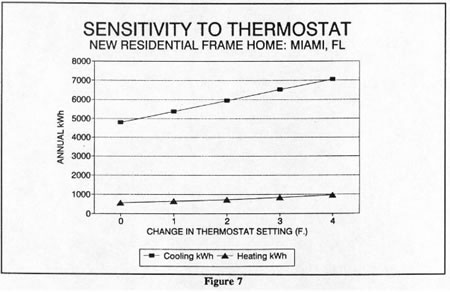
Recent field studies by EPRI of an advanced heat pump lends credence to the theory that "lifestyle" is often expressed as thermostat settings. Thermostat behavior can vary greatly from one home to the next (Lutz, 1992). In the EPRI research differences in the individual thermostat settings in 30 homes being tested accounted for almost all of the variation between the predicted and actual performance of the systems (Kesselring and Lannus, 1991). Use of the DOE 2.1 simulation with the base frame building prototype, showed that a 2oF change in summertime thermostat setting could be expected to alter space cooling energy consumption by approximately 24%. To the extent that "take-back" of comfort is expressed as a changed thermostat setting in response to increased efficiency, we could expect space conditioning savings to be degraded by a like amount. Figure 7 illustrates the sensitivity of the calculated space conditioning loads to increases (heating) or decreases (cooling) to the thermostat setpoint.
Regardless of the immediate reality of the take-back phenomenon, recent studies suggest that its effects may be temporal in many cases, with building owners eventually becoming sensitive once more to utility costs after memory of the alteration fades (Weihl et al., 1988; Keating, 1990).
The relative persistence of savings from energy efficiency measures is another consideration. Service related measures, such as air conditioner tune-ups, may quickly decline in performance whereas others, such as roof coatings, may slowly degrade over a 15-year period. White colored walls may be repainted a darker color. Loss of anticipated savings may be acute in rental properties with equipment installed that requires an informed occupant, such as with a programmable thermostat (Uhlaner and Armstrong, 1991). Still other measures, such a high-efficiency air conditioner change-outs, may experience short-term consumer take-back, with increased savings over the long-run as homeowners realize that monthly utility costs are still sensitive to the degree of use (Rochester Gas and Electric, 1988).
We conclude that while "take-back" and "savings persistence" may
reduce the realized savings of some of the described measures, it is
not a significant enough problem to undermine the more cost-effective
options described in this report. Obviously, however, further research
on this elusive phenomenon is desirable in order to assure available
efficiency savings with greater certainty.
9. Analysis of Technical Savings Potential
Most energy efficiency improvements that reduce air conditioning loads behave according to a law of diminishing returns. The fundamental characteristic is one of decreasing savings associated with each increment designed to reduce building or machine loads. As a result, we analyzed the incremental savings associated with each measure for both new and existing structures using optimization by steepest descent. This means that the measure with the greatest savings is chosen first and implemented in the base case building before re-evaluating the measures for the next choice. Where multiple, competing measures existed (such as with windows), the highest performance option was chosen first to the exclusion of the remaining options associated with the same component. In this way, it is possible to determine a "technical optimum" series of measures. Tables 9 and 10 show the technical optimization process for new and existing homes, respectively. The results are illustrated in Figures 8 and 9.
The technical potential for energy savings in new South Florida homes showed that up to 72% (3,866 kW) of annual heating and cooling electricity consumption could be avoided through incorporation of the fifteen most effective measures. Peak heating and cooling electricity demand could be feasibly reduced by 74% (3.0 kW) and 70% (1.69 kW), respectively.
The analysis of technical savings potential for existing homes indicated that up to 75% (5,366 kW) of annual heating and cooling energy use could be avoided through installation of the fourteen most effective measures. Peak heating electricity demand could be potentially reduced by 63% (3.7 kW). Peak cooling energy demand could be feasibly decreased by 75% (2.49 kW).
The analysis of technical potential does not consider cost. Although a cost-effectiveness analysis is ultimately desirable, we wished to determine the most superior group of performance measures, separate from cost. This is important since the expense of some newer high-technology items is subject to future change. Moreover, measures that currently appear promising, but are too expensive can be targeted for efforts to reduce their cost.
Table 9
Technical Optimization: New Construction
| Measure Description |
Heating kWh |
Cooling kWh |
Total kWh |
Heating Peak kW |
Cooling Peak kW |
| 1. Reference Case | 555 |
4788 |
5344 |
4.03 |
2.43 |
| 2. Advanced Heat Pump | 362 |
3177 |
3538 |
1.76 |
1.61 |
| 3. Dbl-pane, low-E, SS windows | 286 |
2532 |
2818 |
1.38 |
1.32 |
| 4. Ducts Interior | 245 |
2094 |
2339 |
1.18 |
1.09 |
| 5. Reflective Roof | 256 |
1933 |
2189 |
1.18 |
1.02 |
| 6. Landscaping | 271 |
1822 |
2093 |
1.19 |
0.98 |
| 7. Ceiling Fans | 265 |
1651 |
1916 |
1.18 |
0.83 |
| 8. Lower Appliance Gains | 330 |
1419 |
1749 |
1.23 |
0.77 |
| 9. Programmable Thermostat | 312 |
1350 |
1662 |
1.23 |
0.82 |
| 10. R30 Attic | 278 |
1333 |
1611 |
1.17 |
0.80 |
| 11. R19 Walls | 237 |
1317 |
1554 |
1.08 |
0.78 |
| 12. Infiltration Control | 230 |
1303 |
1533 |
1.05 |
0.77 |
| 13. Insulated Duct | 215 |
1301 |
1516 |
1.03 |
0.77 |
| 14. White Walls | 222 |
1282 |
1504 |
1.03 |
0.76 |
| 15. Shade Condenser | 222 |
1256 |
1478 |
1.03 |
0.74 |
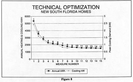
Table 10
Technical Optimization: Existing Homes
| Measure Description |
Heating kWh |
Cooling kWh |
Total kWh |
Heating Peak kW |
Cooling Peak kW |
| 1. Reference Case | 1043 |
6033 |
7076 |
5.92 |
3.31 |
| 2. Advanced Heat Pump | 592 |
3133 |
3725 |
2.42 |
1.70 |
| 3. Window Awnings | 716 |
2524 |
3240 |
2.44 |
1.51 |
| 4. Seal Ducts | 659 |
2208 |
2867 |
2.24 |
1.32 |
| 5. Reflective Roof | 691 |
1925 |
2616 |
2.24 |
1.20 |
| 6. Landscaping | 740 |
1752 |
2492 |
2.25 |
1.16 |
| 7. Ceiling Fans | 729 |
1512 |
2240 |
2.25 |
0.97 |
| 8. Reduce Appliance Gains | 813 |
1321 |
2134 |
2.30 |
0.91 |
| 9. Programmable Thermostat | 763 |
1242 |
2005 |
2.36 |
0.95 |
| 10. Reflective Window Film; E/W | 761 |
1198 |
1959 |
2.35 |
0.92 |
| 11. White Walls | 818 |
1076 |
1893 |
2.36 |
0.89 |
| 12. R-30 Attic Insulation | 761 |
1024 |
1784 |
2.23 |
0.86 |
| 13. Infiltration Control | 754 |
1008 |
1762 |
2.21 |
0.84 |
| 14. Shade Condenser | 754 |
986 |
1740 |
2.21 |
0.82 |
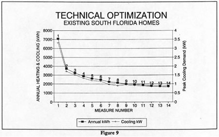
10. Economics of Heating and Cooling Measures
Table 11 shows the economic ranking of the various heating and cooling measures when evaluated on an individual basis. The costs are based on cost data collected for the study and contained in Appendix C and a previous study by Cummings (1988) which examined the expense of many of the considered options. The measures below are ranked by the cost of conserved electricity in dollars per kilowatt hour. Calculation of the cost of conserved electricity is detailed in Appendix G. A nominal discount rate of 10% is used. The cost of conserved electricity allows the savings of the individual measures over their useful life to be compared to the current cost of electricity. Simple payback, a commonly used lay criteria is also computed.
Table 11
Economics of Heating and Cooling Measures for New Construction
| Incremental Measures |
Saved kWh |
$ Cost |
$ Annual Savings |
Simple Pay- back (Yrs.) |
Life (Yrs.) |
CCE ($/kWh) |
| White Walls | 82 |
$0 |
$7 |
0.0 |
30 |
$0.000 |
| Sealed Duct System | 643 |
$225 |
$51 |
4.4 |
20 |
$0.028 |
| Single Pane, Refl.; E/W | 352 |
$170 |
$28 |
6.0 |
20 |
$0.039 |
| Reduce Appl. Gains | 307 |
$125 |
$25 |
5.1 |
15 |
$0.039 |
| Landscaping (mature) | 1092 |
$740 |
$87 |
8.5 |
30 |
$0.044 |
| TDS Interior | 908 |
$725 |
$73 |
10.0 |
30 |
$0.052 |
| Radiant Barrier | 400 |
$325 |
$32 |
10.2 |
30 |
$0.053 |
| Single Pane, Refl. | 731 |
$500 |
$58 |
8.5 |
20 |
$0.055 |
| Hi. Eff. Air Conditioner | 701 |
$400 |
$56 |
7.1 |
15 |
$0.055 |
| Zoned Building | 1317 |
$1,200 |
$105 |
11.4 |
30 |
$0.059 |
| Ceiling to R30 | 228 |
$210 |
$18 |
11.5 |
30 |
$0.060 |
| Programmable T-stat | 226 |
$200 |
$18 |
11.1 |
20 |
$0.071 |
| Refl. Dbl.; E/W Windows | 446 |
$420 |
$36 |
11.8 |
20 |
$0.076 |
| Dbl. Pane Low-E, Refl. | 1025 |
$1,120 |
$82 |
13.7 |
20 |
$0.088 |
| Single Pane, SS | 563 |
$670 |
$45 |
14.9 |
20 |
$0.095 |
| Whole House Fan | 388 |
$470 |
$31 |
15.1 |
20 |
$0.097 |
| Insulated Door | 284 |
$50 |
$2 |
22.0 |
30 |
$0.115 |
| Landscaping (new) | 13 |
$740 |
$33 |
22.4 |
30 |
$0.117 |
| Ceiling Fans | 381 |
$600 |
$30 |
19.7 |
20 |
$0.126 |
| Dbl. Pane Windows | 355 |
$560 |
$28 |
19.7 |
20 |
$0.127 |
| High Eff. Heat Pump | 867 |
$1,200 |
$69 |
17.3 |
15 |
$0.133 |
| Super Eff. Heat Pump | 1806 |
$2,500 |
$144 |
17.3 |
15 |
$0.133 |
| Shade A/C Condenser | 113 |
$250 |
$9 |
27.6 |
30 |
$0.144 |
| Dbl. Pane, Low-E, SS | 1163 |
$2,240 |
$93 |
24.1 |
20 |
$0.155 |
| Reflective Roof | 430 |
$600 |
$34 |
17.4 |
10 |
$0.181 |
| Wall Ins. to R19 | 108 |
$325 |
$9 |
37.5 |
30 |
$0.195 |
| Single Pane, Lam. Low-E | 900 |
$2,240 |
$72 |
31.1 |
20 |
$0.200 |
| Infiltration Control | 91 |
$200 |
$7 |
27.5 |
15 |
$0.212 |
| Window Awnings | 622 |
$200 |
$50 |
40.2 |
15 |
$0.310 |
Table 12
Economics of Heating and Cooling Measures for Existing Housing
| Incremental Measures |
Saved kWh |
$ Cost |
$ Annual Savings |
Simple Pay- back (Yrs.) |
Life (Yrs.) |
CCE ($/kWh) |
| White Walls | 361 |
$0 |
$29 |
0.0 |
20 |
0.000 |
| High Eff. A/C | 1993 |
$400 |
$159 |
2.5 |
15 |
0.019 |
| Sealed Duct System | 764 |
$225 |
$61 |
3.7 |
15 |
0.028 |
| R-19 Attic | 217 |
$110 |
$17 |
6.3 |
20 |
0.041 |
| High Eff. Heat Pump | 2301 |
$1,200 |
$184 |
6.5 |
20 |
0.042 |
| Mature Landscape | 1418 |
$740 |
$113 |
6.5 |
20 |
0.042 |
| Window Film: E/W | 449 |
$250 |
$36 |
7.0 |
20 |
0.045 |
| Reduce Appl. Gains | 345 |
$200 |
$28 |
7.3 |
20 |
0.047 |
| R-30 Attic | 417 |
$300 |
$33 |
9.0 |
20 |
0.058 |
| Programmable T-stat | 321 |
$250 |
$26 |
9.7 |
20 |
0.062 |
| Ceiling Fans | 753 |
$600 |
$60 |
10.0 |
20 |
0.064 |
| Whole House Fan | 530 |
$470 |
$42 |
11.1 |
20 |
0.071 |
| Super Eff. Heat Pump | 3203 |
$2,500 |
$256 |
9.8 |
15 |
0.075 |
| Reflective Roof | 630 |
$500 |
$50 |
9.9 |
10 |
0.103 |
| New Landscape | 551 |
$740 |
$44 |
16.8 |
15 |
0.129 |
| Shade A/C Condenser | 142 |
$250 |
$11 |
21.9 |
20 |
0.141 |
| Infil. Control | 96 |
$200 |
$8 |
26.0 |
20 |
0.167 |
| Awnings | 944 |
$2,000 |
$76 |
26.5 |
20 |
0.170 |
| No Attic Insulation | -1314 |
$1 |
($105) |
0.0 |
20 |
0.000 |
| No Attic/Refl. Roof | 1381 |
$500 |
$110 |
4.5 |
20 |
0.000 |
11. Incremental Economic Analysis for Heating and Cooling
Measures passing the above economic test (CCE < $.08/kWh) were subjected to an incremental analysis to choose those which were cost effective under the most stringent criteria. An incremental analysis is more rigorous since most conservation related improvements are subject to steadily diminishing returns and frequently have strong interactions. Table 13 and Figure 10 shows the analysis results for new construction. The final measure for both new and existing houses reflects the substitution of smaller 2-ton air conditioner after efficiency improvements are made. This measure has a negative cost (saves $400) with positive savings associated with improved part-load efficiency. This option is discussed in Section 12. Table 14 and Figure 11 show the analysis for existing residences.
Table 13
Incremental Economics of Heating and Cooling for New Construction
| Measure Description |
Heating & Cooling
kWh |
Cumulative Savings kWh |
Heating Peak kW |
Cooling Peak kW |
Cumulative $ Cost |
Cumulative CCE ($/kWh) |
| Reference Case | 5344 |
0 |
4.03 |
2.43 |
$0 |
--- |
| White Walls | 5261 |
82 |
4.03 |
2.41 |
$0 |
$0.000 |
| Sealed Ducts | 4629 |
715 |
3.70 |
2.11 |
$225 |
$0.030 |
| Radiant Barrier | 4295 |
1049 |
3.70 |
1.94 |
$525 |
$0.040 |
| SP, Refl. E/W | 3959 |
1384 |
3.73 |
1.77 |
$695 |
$0.040 |
| Reduce Appl. Gains | 3713 |
1631 |
3.88 |
1.68 |
$820 |
$0.040 |
| High Eff. A/C | 3271 |
2073 |
3.88 |
1.44 |
$1220 |
$0.047 |
| Landscape | 3088 |
2256 |
3.91 |
1.36 |
$1960 |
$0.068 |
| Smaller A/C | 2718 |
2625 |
3.91 |
1.29 |
$1560 |
$0.044 |
Measures passing this more stringent test are those which either have a low cost (such as white walls) or those with great effectiveness (such as a high efficiency air conditioner). The package of seven cost-effective measures reduces heating and cooling energy use by 49%. Total package costs are less than $1,600 including the credit for the smaller air conditioner.
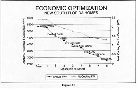
Table 14
Incremental Economics of Heating and Cooling for Existing Residences
| Measure Description |
Heating & Cooling
kWh |
Cumulative Savings kWh |
Heating Peak kW |
Cooling Peak kW |
Cumulative $ Cost |
Cumulative CCE ($/kWh) |
| Reference Case | 7076 |
0 |
5.92 |
3.31 |
$0 |
--- |
| Refl. Roof | 6446 |
630 |
5.94 |
3.02 |
$0 |
$0.000 |
| White Walls | 6112 |
964 |
5.98 |
2.93 |
$0 |
$0.000 |
| High Eff. A/C | 4485 |
2590 |
5.98 |
1.95 |
$400 |
$0.020 |
| Sealed Ducts | 3990 |
3085 |
5.49 |
1.71 |
$625 |
$0.030 |
| Reduce Appl. Gains | 3862 |
3213 |
5.63 |
1.65 |
$750 |
$0.033 |
| Pr. T-stat | 3664 |
3411 |
5.64 |
1.70 |
$950 |
$0.037 |
| W. Film: E/W | 3420 |
3656 |
5.52 |
1.58 |
$1200 |
$0.044 |
| Landscape | 3269 |
3807 |
5.56 |
1.51 |
$1940 |
$0.057 |
| Smaller AC | 2953 |
4123 |
5.56 |
1.37 |
$1540 |
$0.043 |
Nine measures were found cost-effective for existing buildings. Of these, change to a high-efficiency air conditioners (SEER 12.0) provides a large fraction of the 58% annual heating and cooling energy savings. Total package cost is approximately $1,500.
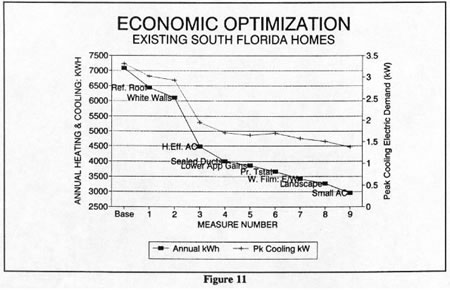
12. Peak Load Reduction and Air Condtioner Sizing
Many of the more successful energy efficiency measures have a very beneficial impact on the daily peak electrical demand. Reduction to peak demand is quite beneficial to Florida utilities. Often the peak utility demand occurs from 2 to 6 PM during the summer when temperatures and solar gain are greatest. Generally, maximum summertime FPL system loads occur at about 5:30 PM daily. Figure 12 shows the monitored AC load shape in 58 homes with central AC in 1988 over the five hottest days of summer. Superimposed are the DOE-2 predicted loads for August 1st for the existing and new home prototypes. Although, somewhat lower during nighttime hours, the predicted AC loads for the existing house prototype corresponds very well with the measured data. The timing of the winter utility system peak is more variable, sometimes occurring during morning hours and at other times during the evening hours (Taylor, 1990).
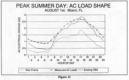
Field studies have shown that residential air conditioners are frequently over-sized (Lucas, 1992). Conversations with air conditioning contractors in the Miami area revealed that large air conditioners, frequently four tons or greater for residential applications, are frequently installed. Installers indicated that simple rules of thumb are often used for residential sizing. Over-sizing has been shown to be among the most significant factors in affecting residential air conditioning electrical demand at utility coincident peak (Neal and O'Neal, 1992). The later study showed that proper sizing of air conditioners relative to common practice (75% over-sized) would reduce utility peak demand by some 23%. Other work has shown that proper air conditioning sizing leads to greater occupant comfort through improved dehumidification (Katipalmula et al., 1988).
Based on the collected cost data, we determined that each additional ton of air conditioning capacity has a cost of some $300 - $500-- depending on machine efficiency. Improvements to the building envelope and the thermal distribution system provide large potential impacts to the required size of the air conditioning system. Our base analysis, using procedures outlined in Chapter 26 of the Handbook of Fundamentals showed that a three ton air conditioner would be required for our new frame prototype residence (ASHRAE, 1989).
The same analysis performed after a reflective roof or radiant barrier was installed along with improved east and west windows, lower appliance gains and landscaping was installed showed that the recommended cooling machine size had dropped to two tons in capacity. Not only would proper sizing result in reduced energy and peak demands, but also in improved household comfort at a lower initial cost. As a consequence, we recommend that a standard air conditioner sizing procedure be used for any reconstruction in the Miami area.
The economically optimal package of measures for new construction reduced peak cooling energy use by 1.14 kW or some 47%. The chosen package for existing buildings reduced the AC peak demand by 1.94 kW or 59%. Peak savings were higher for existing residences due to the large improvement in achieved air conditioning efficiency from the conservation package. In either case, down-sizing of the air conditioner after efficiency improvements to the building have been made, is instrumental to much of the reduction.
13. Water Heating
Based on the current study of DSM potential in the state of Florida, residential water heating represents nearly 10,000 GWh of the 71,000 GWh of electricity used annually (SRC, 1992). According to the same study, the average South Florida household uses 2,134 kWh per year to heat water at an overall cost of $170. This 14% of overall residential energy use is amenable to significant reductions with readily available off-the-shelf technologies. Conservation options tend to be inexpensive. Also, when low-cost conservation measures are incorporated, the water heating loads drop to the extent that alternative water heating technologies can easily provide a large fraction of the overall remaining demand. We briefly summarize the various methods, their savings and costs.
Conservation
Available conservation measures include better insulated tanks, low-flow showerheads, external water heater tank wraps and pipe insulation and anti-thermosiphon heat traps. The savings for better insulated tanks can be computed from the differences in the energy-factor (EF) rating of the units. Because of the 1990 National Appliance Efficiency Standards, newer water heaters are more efficient. A typical new 40 gallon tank, the most common size in Florida households, will typically have an energy factor of 0.88. However, better insulated tanks of the same capacity are now available with EFs of 0.95 or better. This means approximately a 7% savings in water heating energy use or approximately 149 kWh. The $130 added cost of such unit is based on data from a national vendor (Sears, 1992). The savings for the other water heating conservation measures is taken from a recent LBL study (Koomey et al., 1991):
Table 15
Water Heating Conservation Measures
Measure Description |
Percent Savings |
Saved kWh |
Cost $ |
Life (Yrs) |
| High Efficiency Tank | 7% |
149 |
$135 |
13 |
| Low-flow Showerheads | 10% |
213 |
$20 |
10 |
| External Tank Insulation | 9% |
192 |
$90 |
14 |
| Pipe Insulation/Heat Trap | 3% |
64 |
$30 |
13 |
Heat Pump Water Heaters
Heat pump water heaters use the carnot cycle to improve the electrical efficiency with which domestic hot water is produced. Merrigan (1990) found an overall coefficient of performance (COP) for heat pump water heaters of 1.53 in a field study of 16 units in Florida in 1982-1984. Other field studies for Florida Power and Light and Gulf Power found field COPs of 1.77 and 2.00, respectively (ORNL, 1981). We take a simple average of the three studies for our analysis (COP = 1.77). When compared to the overall COP of resistance units in Merrigan's study, this results in a fractional savings of 54% or 1,152 kWh. Based on data collected by FSEC, we estimate the cost of an integral heat pump water heater at approximately $1,500. Small add-on units (which use the existing tank) costing only $600 are available. These have estimated water heating energy savings of about 30% (Koomey et al., 1991). This indicates a savings for these add-on units of some 640 kWh.
Solar Water Heaters
The savings potential of solar water heaters in Florida has been well researched. Merrigan's study of 20 Florida solar water heating systems in 1982 found an average coefficient of performance of 2.35 relative to 0.82 for 18 electrical resistance systems. This implies a 65% reduction in electrical use relative to standard water heaters. More modern units offer improved reliability and performance at a lower expense. In the past, solar water heaters typically had costs from $1,500 -$3,000 installed. Our standard solar hot water system assumes a larger 4 x 10 foot collector with an 80 gallon storage tank. We estimate an 80% solar fraction for such a system and a cost of $2,250 installed.
An important innovation, however, is the availability of a new low-cost solar water heater. The system with a 2 x 10' collector sells for only $700. It is designed to provide 95% of water heating for a household of two and 50% for a home with four members. Although it can be self-installed, professional installation is assumed to add $350 to the price. Savings should average approximately 70% in a three person household. This formed the basis for the estimated savings in the Miami for an add-on system of 1,494 kWh. Test results are available from the Florida Solar Energy Center.
Summary of Water Heating Measures
The economics of the various water heating measures is summarized in Table 16. Utility coincident peak load savings are based on field monitoring of resistance, heat pump, desuperheater and solar water heating systems (Merrigan and Parker, 1990). Peak savings for the conservation measures were estimated by applying the savings fractions in Table 15 to the measured diversified summer (0.54 kW) and winter peaks (1.20 kW) from the same study.
Table 16
Water Heating Measures
Saved kWh |
Winter Peak Demand Savings (W) |
Summer Peak Demand Savings (W) |
Cost $ |
Annual Savings $ |
Simple Payback (Yrs.) |
Life (Yrs.) |
CCE ($/kWh) |
|
| Conservation Measures | ||||||||
| Low-head showers | 213 |
120 |
54 |
$20 |
$40 |
2.3 |
10 |
$0.024 |
| External tank insulation | 192 |
108 |
49 |
$90 |
$15 |
5.9 |
13 |
$0.050 |
| Pipe insulation/heat trap | 64 |
33 |
16 |
$30 |
$5 |
5.9 |
13 |
$0.050 |
| High efficiency tank | 149 |
77 |
37 |
$130 |
$12 |
10.9 |
13 |
$0.096 |
| Alternative Water Heating Systems | ||||||||
| Add-on solar water heater | 1494 |
580 |
430 |
$1050 |
$120 |
8.7 |
15 |
$0.068 |
| Add-on hp water heater | 640 |
340 |
30 |
$600 |
$51 |
11.7 |
15 |
$0.090 |
| Heat recovery water heater | 811 |
230 |
380 |
$800 |
$65 |
12.3 |
15 |
$0.095 |
| Heat pump water heater | 1152 |
610 |
50 |
$1500 |
$92 |
16.3 |
15 |
$0.125 |
| Standard solar water heater | 1707 |
660 |
490 |
$2250 |
$137 |
16.5 |
20 |
$0.127 |
Our analysis showed that most of the various water heating conservation measures are cost-effective. However, only the add-on solar water heater is a cost effective alternative system to resistance water heating.
14. Refrigeration
Refrigeration is generally the third largest end-use of energy in South Florida homes. Total consumption for refrigerators and freezers in the state is estimated at approximately 12,800 GWh, or approximately 18% of overall residential energy consumption. There are at least seven million refrigerator-freezers in operation in Florida. Best estimates are that auto-defrost refrigerators in South Florida use about 1,770 kWh (SRC, 1992). Not only do these refrigerators directly use electricity, they also add heat to the interior of Florida homes, increasing the need for air conditioning.
Approximately 25% of these refrigerators are old, inefficient and awaiting replacement. Two field studies of measured refrigerator energy use have been conducted in the state. One monitoring program of 25 homes in Palm Beach County showed that the average household used 3,730 kWh for refrigeration -- 15% of overall electricity use (Messenger et al., 1982). A number of the homes had second refrigerators or freezers. Fifteen units were replaced with more efficient models resulting in an average post-retrofit savings of 33%. Another case study of refrigerator replacement was recently performed by FSEC (Parker and Stedman, 1992). The existing, 1975 vintage refrigerator and a new, more efficient unit were each monitored over an entire year. The newer unit was found to reduce refrigerator electrical consumption by nearly 60%, a savings of 1,200 kWh per year. This illustrates how electricity savings from replacement of older refrigerators can be potentially significant.
More efficient units are becoming available as the 1993 appliance efficiency standards take effect. The average unit manufactured in 1992 used about 1,000 kWh. Of these, some models are inherently more efficient than others. Side-by-side units, particularly those with through-the-door (TTD) features have been measured to use 10 - 40% more electricity than others (Ross, 1991; Parker and Stedman, 1992). Although convenient, these units also cost more to purchase. A listing of the most efficient units of a given size and type can be obtained from the 1992 Consumer Selection Guide for Refrigerators and Freezers or in the Consumer Guide to Home Energy Savings (AHAM, 1992; Wilson and Morrill, 1992). Future improvements to refrigerators will likely lead to additional savings for this measure.
High efficiency refrigerator options for South Florida are summarized in Table 17. It is assumed that the units for an existing home would be replaced outright. Savings for new housing reflect the incremental choices relative to a conventional, new 1,000 kWh per year unit. Based on field monitoring, the utility peak coincidence of refrigerators is assumed to be 120% in summer and 90% of average consumption in winter (Parker and Stedman, 1992).
Table 17
Refrigerator Efficiency Measures
| Measure Description | Percent Savings |
Saved kWh |
Saved Winter Peak (W) |
Saved Summer Peak (W) |
Cost $ |
Simple Payback (Yrs.) |
Life (Yrs.) |
CCE ($/kWh) |
| Existing Housing | ||||||||
| Replace older unit (<1980) with same size model |
40% |
710 |
73 |
97 |
$600 |
10.6 |
15 |
$0.081 |
| As above, but avoid side-by-side and TTD features | 50% |
880 |
91 |
121 |
$500 |
7.1 |
15 |
$0.055 |
| New Housing | ||||||||
| Choose most efficient unit for size | 10% |
100 |
11 |
14 |
$50 |
6.3 |
15 |
$0.048 |
| Choose most efficient unit for size; avoid side-bye-side and TTD features | 20% |
200 |
20 |
27 |
$0 |
0.0 |
15 |
$0.000 |
15. Lighting
At 1,000 kWh per year, indoor lighting represents a relatively small fraction (7%) of the average household electrical consumption in South Florida. However, this is a portion of energy use that can be substantially reduced through the substitution of new compact fluorescent lamps (CFLs) (Parker and Drake, 1991). More efficient halogen incandescent lamps can be substituted into fixtures which will not otherwise accommodate CFLs. The average Florida home has approximately 28 lamp fixtures, the majority of which use common incandescent lamps. These lamps are inexpensive, but very inefficient -- typically only about 10% of the electricity used is converted to visible light. The rest is converted to waste heat, which makes the air conditioner work longer. Incandescent bulbs produce about 17 lumens per watt of input electricity; the newer compact fluorescent lamps produce about 50 lumens per watt. Also, unlike older cool-white fluorscents, the new generation of CFLs have better color-rendering attributes; the light they cast looks very similar to that from a conventional incandescent bulb.
A CFL substitute lamp for a 75 Watt incandescent bulb only uses about 18 Watts. These lamps last about ten times as long as the average incandescent bulb (10,000 vs. 1,000 hours). A variety of different type of CFLs are available to substitute into existing fixtures. Utility studies have shown that approximately 30% of fixtures in existing homes can be converted to CFLs (Delta-T, 1990). The potential fraction in new homes is certain to be greater since the fixtures can be designed to accommodate the more efficient lamps. CFLs are, however, fairly expensive at $10 - $25 each. Because of their cost they should only be used in fixtures where they will be operated more than about two hours per day. We conservatively assume that 10 fixtures can be converted to CFLs in new dwellings, and half this many in existing homes. Lamps in which CFLs are located are operated three hours per day. This involves targeting of frequently used lamps. As a conservatism, we assume that lighting measures produce no coincident peak electrical savings.
Halogen incandescent bulbs represent a more efficient incandescent lighting technology with excellent color rendering qualities. The bulbs are also nearly identical in size to standard bulbs and can be readily substituted into most fixtures. The halogen lamps last about three times as long as standard bulbs and cost about $2 - $3 each. They are cost effective to install in lamps that are used a hour a day or more. We assume that five fixtures in new homes would qualify for such lamps and ten in existing homes where CFLs may be harder to substitute because of fixture dimensions.
Table 18
Lighting Measures
| Measure Description |
Hrs/ Day |
Saved kWh |
Cost $ |
$ Annual Savings |
Simple Payback (Yrs.) |
Life (Yrs.) |
CCE ($/kWh) |
| New Housing | |||||||
| (10) 75W-> 18W CFL (5) 75W-> 52W Halogen |
3 hr 1 hr |
630 42 |
$150 $15 |
$50 $3 |
3.0 4.5 |
8.2 9.6 |
$0.036 $0.048 |
| Existing Housing | |||||||
| (5) 75W-> 18W CFL (10) 75W-> 52W Halogen |
3 hr 1 hr |
315 84 |
$75 $30 |
$25 $7 |
3.0 4.5 |
8.2 9.6 |
$0.036 $0.048 |
Our analysis indicates both CFLs and halogen incandescent lamps are cost-effective in residential applications. Up to 67% of lighting energy use in new housing can be avoided. About 40% of lighting electricity use in the existing houses can be reduced through use of these technologies.
16. Swimming Pool Pumps
About 24% of South Florida homes have swimming pools. Pool pumping is very energy intensive. The average pool pump uses about 3,120 kWh per year (SRC, 1992; Messenger et. al., 1982). Pumps are frequently oversized with narrow piping and small filters. They also may be operated more frequently than necessary. The average pool pump runs about eight hours a day. A detailed experimental study of 120 pools by Florida Atlantic University found that pool pump operation no more than four hours per day resulted in no degradation in pool clarity or increase in algae formation (Messenger and Hays, 1982).
Pump, piping and filter sizing are strong determinants of pool circulation efficiency. Generally, a small pump with large piping and an oversized filter will significantly reduce energy consumption. The National Pool and Spa Institute recommends 1/2 horsepower pumps be used with pools of up to 20,000 gallon capacity; 3/4 horsepower pumps are recommended for pools up to 28,000 gallons (National Pool and Spa Institute, 1992). Two-inch plumbing and larger filter sizing (36 square feet diatomaceous earth (DE) filter; 70 sq ft cartridge or 24" high-rate filter) will further increase circulation efficiency.
For instance, a 1/2 hp pump with 2-inch piping and a larger filter substituted for a 1 hp pump with 1.5-inch piping could be expected to provide a similar level of flow under typical conditions (Messenger and Hayes, 1986). Running the efficient system for 4 hours per day would use an estimated 1,050 kWh per year as opposed to 3,310 kWh for the less efficient system run for eight hours daily. The incremental cost of a smaller pump with larger piping and a larger filter is approximately $50 for the average residential application. A pool pump timer is assumed to cost $100 installed for a existing installation. Change-out to a smaller pump for an existing installation is assumed to cost $350 installed. All analyzed measures were extremely cost-effective with paybacks of two years or less.
Table 19
Pool Pump Measures
| Measure Description |
Hrs/ Day |
Saved* kWh |
Peak Demand Savings (W) |
Cost $ |
Annual Savings $ |
Simple Payback (Yrs.) |
Life (Yrs.) |
CCE ($/kWh) |
| New Housing | ||||||||
| 1/2 hp pump with 2" piping and oversized filter | 4 hr |
2,260 |
85 |
$50 |
%181 |
0.3 |
10 |
$0.003 |
| Existing Housing | ||||||||
| Add pump timer | 4 hr |
1,655 |
62 |
$100 |
$133 |
0.8 |
10 |
$0.008 |
| Change to 3/4 hp pump | 4 hr |
1,870 |
70 |
$350 |
$150 |
2.3 |
10 |
$0.010 |
* Base case assumes 1 hp pump
with 8 hours of daily operation. |
||||||||
Peak load savings are based on a 33% level of diversified pool pump demand coincidence with the utility system peak. This is very conservative since the base eight hours of pool pump operation are more likely to be concentrated during daytime hours (7 AM - 6 PM) when the winter and summer peak often occurs.
17. Economic Analysis of All End-Use Measures
Our final analysis examined all measures competing against each other to determine their relative economic ranking. As before, the cost of conserved electricity was used for the analysis. Interactions were taken into account through computer simulation of the measures incorporated into the building in an incremental fashion. The heating and cooling measures were grouped into two "packages" summarized in Table 13 and 14. Table 20 and Figure 13 show how overall building energy use in new residences is reduced as measures are added in an incremental fashion. Table 21 and Figure 14 show the same analysis for existing residences.
Table 20
Overall Economic Optimization in New South Florida Residences
| Measures | Saved kWh |
Total kWh |
CCE ($/kWh) |
Cumulative CCE |
Cost $ |
Cumulative $ Cost |
| 1. Reference Case | 0 |
16143 |
$0.000 |
--- |
$0 |
$0 |
| 2. Smaller Pool Pump | 2260 |
13883 |
$0.003 |
$0.003 |
$50 |
$50 |
| 3. DHW: Showerheads | 213 |
13670 |
$0.024 |
$0.006 |
$40 |
$90 |
| 4. Lights: CFLs | 630 |
13040 |
$0.036 |
$0.013 |
$150 |
$240 |
| 5. Heating and Cooling Pkg. | 2625 |
10415 |
$0.044 |
$0.028 |
$1560 |
$1800 |
| 6. Lights: Halogen | 42 |
10373 |
$0.048 |
$0.028 |
$15 |
$1815 |
| 7. H. Eff. Refrigerator | 100 |
10273 |
$0.048 |
$0.029 |
$50 |
$1865 |
| 8. DHW: Ext. Tank Ins. | 192 |
10081 |
$0.050 |
$0.029 |
$90 |
$1955 |
| 9. DHW: Pipe Insulation | 64 |
10017 |
$0.050 |
$0.030 |
$30 |
$1985 |
| 10. DHW: Add-on Solar | 1494 |
8523 |
$0.068 |
$0.038 |
$1050 |
$3035 |
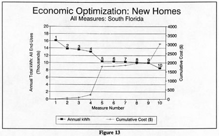
Table 21
Overall Economic Optimization in Existing South Florida Residences
| Measures | Saved kWh |
Total kWh |
CCE ($/kWh) |
Cumulative CCE |
Cost $ |
Cumulative $ Cost |
| 1. Reference Case | 0 |
18640 |
$0.000 |
--- |
$0 |
$0 |
| 2. Smaller Pool Pump | 1870 |
16771 |
$0.010 |
$0.010 |
$350 |
$350 |
| 3. DHW: Showerheads | 213 |
16558 |
$0.024 |
$0.011 |
$40 |
$390 |
| 4. Lights: CFLs | 315 |
16243 |
$0.036 |
$0.015 |
$75 |
$465 |
| 5. Heating and Cooling Pkg. | 4123 |
12120 |
$0.043 |
$0.033 |
$1540 |
$2005 |
| 6. Lights: Halogen | 84 |
12036 |
$0.048 |
$0.033 |
$30 |
$2035 |
| 7. DHW: Ext. Tank Ins. | 192 |
11844 |
$0.050 |
$0.033 |
$90 |
$2125 |
| 8. DHW: Add-on Solar | 1494 |
10350 |
$0.068 |
$0.040 |
$1050 |
$3175 |
| 9. High Eff. Refrigerator | 710 |
9640 |
$0.081 |
$0.043 |
$600 |
$3775 |
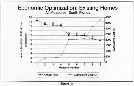
Results show that reductions to annual electricity use of approximately 45% is technically and economically feasible in new and existing homes in South Florida. Energy savings would be approximately 35% in homes without swimming pools. The total savings of approximately 8,000 kWh per year is obtained through a combination of comprehensive measures that reduce electricity use for most end-uses. The overall investment is about $3,400 for new and $4,200 for existing homes. Simple payback is about six years for the package of measures for new and existing homes. The investment performance corresponds to an after-tax rate of return of about 16%.
18. Summary Recommendations
The fundamental purpose of this study was to determine the critical elements that will improve the energy efficiency of reconstructed housing in South Florida. A number of promising measures were identified that together have the technical potential to reduce household energy use by up to 70%. As example, we found that improvements to the building envelope, heating and cooling system, and appliances were technically capable of reducing the space conditioning loads by 73 - 84% in new and existing homes respectively.
However, the economic potential was much lower than the technical potential. Cost-effective options were identified which were able to reduce annual household electricity use by 39 - 48%. The maximum cost effective level for consumers was less than the current cost of electricity ($0.08/kWh). For new homes, we assume that all levels of insulation and equipment efficiency are already installed according to the current state energy code. The measures for existing housing were similar to those for new construction, with the obvious lack of feasibility of some measures (added wall insulation, duct system within the conditioned space). Economically superior measures are summarized below. Figure 15 graphically depicts many of the features of such energy-efficient housing.
Recommended Measures: New Housing
Envelope:
-
Attic radiant barrier or reflective roof
-
Single-pane reflective east and west windows
-
White colored walls
Heating and Cooling System:
-
Sealed duct system
-
Duct system within the conditioned space, attic radiant barrier or reflective roof
-
Air conditioner with SEER > 12.0
-
Proper AC sizing
Water Heating
-
Low flow showerheads
-
Extra hot water tank insulation
-
Add-on solar water heater
Appliances
-
Most efficient refrigerator for size and type
-
Compact fluorescent lighting
-
Halogen incandescent lighting
-
Down-sized pool pump with oversized piping and filter
-
Pool-pump timer
Synopsis: The identified package of measures for new construction in South Florida is capable of cost-effectively reducing annual electricity consumption by 47% for homes with pools (7,600 kWh). Residences without pools can realize savings of 39% or 5,350 kWh. In either case, the efficiency package costs about $3,000. Savings in annual utility costs range from $430 to $600. Simple paybacks are about seven years for homes without pools and about five years for homes with them. Economic performance, corresponding to 14% - 20% after-tax rate-of-return, is very attractive relative to conventional investments. The package saves electricity at a cost of $0.038/kWh. This is less than half of the current retail price of residential electric service. Utility coincident summer peak loads could be reduced by approximately 1.5 kW or about 37%.
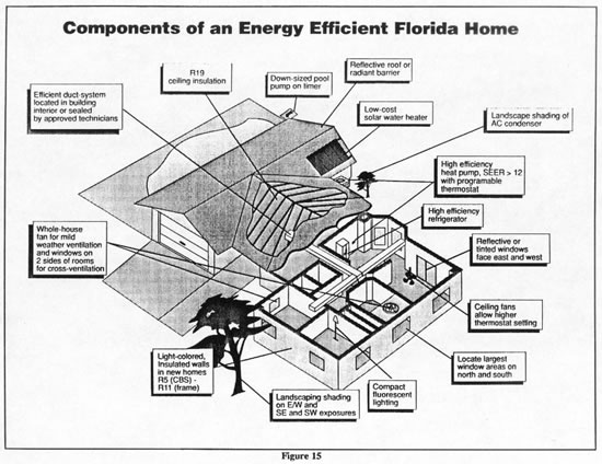
Recommended Measures: Existing Housing
Envelope:
-
Reflective roof or attic radiant barrier if feasible
-
White colored walls
-
Reflective window film on east and west windows
Heating and Cooling System:
-
Air conditioner with SEER > 12
-
Proper AC sizing
-
Sealed duct system
-
Programmable thermostat
Water Heating
-
Low flow showerheads
-
Add-on solar water heater
Appliances
-
Replace older refrigerators
-
Compact fluorescent lighting
-
Halogen incandescent lighting
-
Down-sized pool pump
-
Add pool pump timer
Synopsis: The identified package of measures for existing South Florida homes is capable of cost-effectively reducing annual electricity consumption by 48% for homes with pools (9,000 kWh). Residences without pools can realize savings of 42% or 7,100 kWh. The efficiency package costs about $3,800 for homes with pools and about $3,400 for those without. Savings in annual utility costs range from approximately $570 to $720. Simple paybacks are about six years for homes without pools and about five years for homes with them. Economic performance, corresponding to 14% - 17% after-tax-rate-of-return, is very attractive relative to conventional investments. The package saves electricity at a cost of $0.049/kWh. This is less than half of the current average retail price of residential electric service. Summer utility coincident peak loads are predicted to be reduced by mor than 25 kW.
19. Potential Follow-Up Action
This study finds significant potential for improvements in energy efficiency in rebuilding South Dade residences damaged by Hurricane Andrew. Assuming that the potentials determined in this report are reasonably accurate, each of the 85,000 rebuilt homes could realize annual electricity savings of 5,000 kWh or more. Utility peak loads from these homes could be reduced by up to 50%, or by approximately 2 kW each. Were even half of the rebuilt homes made more efficient, this could account for a reduction in utility capacity of over 80 peak MW and an annual energy savings of upwards to 200,000 MWh.
The direct cost of improving the energy efficiency of the 85,000 homes would be approximately $300 million. Assuming 50% administrative and overhead costs, the overall improvements could be accomplished for approximately $450 million.
However, before launching into a comprehensive program of retrofits, experience has shown that a more limited research pilot program often makes an eventual larger program more effective and cost effective. We therefore recommend that two samples of rebuilt houses be enlisted in such a research program. As envisioned here, 400 rebuilt homes in South Dade would be monitored in the project. Each home would have the following electrical end-uses monitored in addition to detailed audit data taken on each:
-
Heating and cooling
-
Water heating
-
Refrigerator
-
Total
Meteorological data would also be taken on interior temperature and humidity at each site. Centrally located sites would be used to collect representative meteorological data (temperature, humidity, solar radiation, wind speed and direction and rainfall).
Two hundred of the homes would be "current practice" construction, built to the state energy code, but without specialized energy saving options. These would comprise the control group. The other 200 homes would comprise the experimental group. These homes would have selected measures installed in each, using the experimental technique of orthogonal arrays. Orthogonal arrays allow for efficient statistical determination of the influence of each of the selected experimental treatments and associated interactions (Diamond, 1989). The chosen "treatments" for the orthogonal arrays would be as follows:
-
Envelope measures
-
HVAC measures
-
Water heating conservation measures
-
Solar water heating/heat recovery water heaters
-
Refrigerator measures
-
Lighting measures
-
All measures
An illustration of the application of the orthogonal array concept to the proposed experiment is shown in Table 22.
Table 22
Example Orthogonal Array for Residential Energy Efficiency Study
Cell No. |
Envelope System |
HVAC System |
DHW Conserve Measures |
Solar DHW System |
Refrig. Measures |
Lighting Measures |
Block Construction |
1 |
1 |
0 |
0 |
0 |
1 |
0 |
0 |
2 |
1 |
1 |
0 |
0 |
0 |
1 |
0 |
3 |
1 |
1 |
1 |
0 |
0 |
0 |
1 |
4 |
1 |
1 |
1 |
1 |
0 |
0 |
0 |
5 |
0 |
1 |
1 |
1 |
1 |
0 |
0 |
6 |
1 |
0 |
1 |
1 |
1 |
1 |
0 |
7 |
0 |
1 |
0 |
1 |
1 |
1 |
1 |
8 |
1 |
0 |
1 |
0 |
1 |
1 |
1 |
9 |
1 |
1 |
0 |
1 |
0 |
1 |
1 |
10 |
0 |
1 |
1 |
0 |
1 |
1 |
1 |
11 |
0 |
0 |
1 |
1 |
0 |
1 |
0 |
12 |
1 |
0 |
0 |
1 |
1 |
0 |
1 |
13 |
0 |
1 |
0 |
0 |
1 |
1 |
0 |
14 |
0 |
0 |
1 |
0 |
0 |
1 |
1 |
15 |
0 |
0 |
0 |
1 |
0 |
0 |
1 |
16 |
1 |
1 |
1 |
1 |
1 |
1 |
1 |
17 |
1 |
1 |
1 |
1 |
1 |
1 |
0 |
Notes: 1 = Building contains
options; 0 = Building does not contain options |
|||||||
An essential feature of the proposed research program would be that it would not leave the selection of measures to the choice of home owners or builders. Such self-selection and bias along with the natural variation in residential energy use could easily make it impossible to separate out the influences of the various measures. This would, in turn, make potential improvements to the overall efficiency package impossible to discern from the experimental results. We recommend that the various measures, required for each house in the orthogonal array, be installed to home-owners free of charge. In this way it would be possible to obtain superior and unbiased research information at the lowest possible cost.
The overall expense of installing the measures in the 200 homes would be approximately $1 million. The cost of monitoring the 400 homes in the project would likely total approximately $5 million after data acquisition and analysis expenses are included. Likely funding roles for the involved parties might consist of Florida Power and Light Company bearing the cost of the project monitoring and administration with the cost of the energy-efficiency improvements being provided by the U.S. Department of Energy either alone or in concert with We Will Rebuild.
Pursuing the research in this way it would be possible to evaluate each of the program elements, as well as the overall package of measures. Each of the first 16 "cells" (rows) in the array would have 10 houses chosen, with 40 homes in the final "all measures" cell. Each home in the experimental group would have a "matched pair" home in the control group within the same subdivision development. This would help to control for construction-related differences within the various developments.
The research objectives for the pilot study would be to establish the influences of the various experimental treatments and the overall efficiency package on the following variables of interest:
-
Annual electricity use
-
Utility coincident winter peak load
-
Utility coincident summer peak load
The monitoring would be carried out over at least a year long period. Results from the pilot research project would then allow verification or modification to the proposed energy savings packages. With greater confidence in the level of savings to be achieved, the utility program could then be confidently expanded to include all homes, both in the area affected by Hurricane Andrew, as well as the rest of Central and South Florida.
Research results could potentially be available from the research pilot as early as 1995. Since the rebuilding effort in South Dade County will likely take ten years or more, the proposed approach would still allow energy efficiency to be comprehensively addressed during much of the rebuilding effort while gaining valuable experience with the technologies. Such information would also allow Florida's utilities to confidently pursue available residential DSM opportunities into the next decade.
20. Acknowledgements
This work represents a uniquely cooperative effort to effect a positive response to a regional tragedy. Support has been provided by the U.S. Department of Energy (DOE), the Florida Energy Office (FEO) and the Florida Power and Light Company (FPL). Special thanks to Buddy Jackson, Director of the Atlanta DOE Support Office and Jim Tait, Director of FEO. Nelson Hawk, Director of Market Planning, Patrick James, Product Manager, and Sharyn Barata, Associate End-Use Research Coordinator with FPL were all instrumental in supplying data and project support. The generous assistance of each of these agencies in sponsoring this research is gratefully acknowledged. Art Rosenfeld at Lawrence Berkeley Laboratories and John Parker at Florida International University have also provided assistance and encouragement. Doug Yoder and Susan Berryman with the Metro-Dade County Department of Environmental Resources Management have helped to guide the focus of of the effort. BD Publishing, Inc. gratefully provided permission for use to use the color photographs of Hurricane Andrew and its aftermath. At the Florida Solar Energy Center, our director, Dr. David Block, has lent special priority to our work. Last, but not least, Wanda Dutton has very capably assisted with the imposing job of preparing this report.
21. References
Abrams, D.W., Low Energy Cooling, Van Nostrand Rheinhold, New York, 1986.
AEC, Engineering for Estimating the Impacts of Demand Side Management Programs, Vol. 1, Architectural Energy Corp. prepared for Electric Power Research Institute, EPRI-TR-100984s, Palo Alto, CA, July, 1992.
Akbari, H., Davis, S., Dorsano, S., Huang, J. and Winnett, S. Cooling Our Communities: A Guidebook on Tree Planting and Light-Colored Surfacing, 22P-2001, U.S. Environmental Protection Agency, Washington D.C., January, 1992.
AHAM, "1992 Consumer Selection Guide for Refrigerators and Freezers," Association of Home Appliance Manufacturers, Chicago, IL, 1992.
Anderson, R.W., Yarbrough, D.W., Graves, R.S. and Wendt, R.L. "Preliminary Assessment of Radiation Control Coatings for Buildings," Insulation Materials: Testing and Applications, 2nd Volume, ASTM STP 1116, R.S. Graves and D.C. Wysocki, Eds., American Society for Testing and Materials, Philadelphia, 1991.
Andrews, J.W., "Optional Forced Air Distribution in New Housing," Proceedings of the 1992 Summer Study on Energy Efficiency in Buildings, Vol. 2, American Council for an Energy Efficient Economy, Washington, DC, August, 1992.
ASHRAE, Handbook of Fundamentals, American Society of Heating, Refrigeration and Air Conditioning Engineers, Atlanta, GA, 1989.
Al-Mofeez, I. and Woods, P.K., "Experimental Test Results of Interior vs. Exterior Insulation in Extremely Hot Climates," Insulation Materials: Testing and Applications, 2nd Volume, ASTM STP 1116, R.S. Graves and D.C. Wysocki, Eds., American Society for Testing and Materials, Philadelphia, 1991.
Bretz, S., Akbari, H., Rosenfeld, A. and Taha, H., "Implementation of White Surfaces: Materials and Utility Programs," LBL-32467, Lawrence Berkeley Laboratory, Berkeley, CA.
Buffington, D.E., Sastry, S.K. and Black, R.J. Factors for Determining Shading Patterns in Florida: Miami and Vicinity, Circular 512, Florida Cooperative Extension Service, University of Florida, Gainesville, FL, 1981.
Buhl, F. and Hirsch, J. 1987. Building Energy Performance Analysis Using the DOE - 2 Computer Program, Lawrence Berkeley Laboratory, DOE 2.1C Documentation Package, Berkeley, CA, August, 1987.
Burch, D.M. and Treado, S.J., "Ventilating Residences and their Attics for Energy Conservation," in Summer Attic and Whole House Ventilation, NBS Special Publication 548, National Bureau of Standards, Washington D.C., 1979.
Burns, R. and Hough, R.E. Monitoring and Evaluation of Replacing Low-Efficiency Air Conditioners with High-Efficiency Air Conditioners in Single-Family Detached Houses in Austin, Texas, ORNL/Sub/86-SA566/V, Oak Ridge National Laboratories, Oak Ridge, TN, August, 1991.
Chandra, S. and Moalla, S., "Energy Savings from Industrialized Housing Construction Systems and and Roofing Tiles," presented at the Energy Efficient Building Association Conference, Raleigh, NC, March 1992.
Cummings, J.B., The Economics of Energy Saving Features in Home Construction,
FSEC-PF-199, Florida Solar Energy Center, Cape Canaveral, FL, 1988.
Cummings, J.B., J.J. Tooley and Moyer, N. Investigation of Air Distribution System Leakage and Its Impact in Central Florida Homes, FSEC-CR-397-91, Florida Solar Energy Center, Cape Canaveral, FL, January, 1991.
Cummings, J.B., J.J. Tooley and N. Moyer. Florida Fix Weatherization Training Manual, FSEC- GP-42-89, Florida Solar Energy Center, Cape Canaveral, FL, October, 1989.
Davis, W.L. and Adams, R.W., "Energy Management in Residential Building Design in Florida: The Impacts of New Design Strategies on Florida Housing Trends," Proceedings of the World Congress on New Trends in Housing Projects, Florida Power and Light Company, Miami, FL, December, 1986.
Diamond, W. J., Practical Experiment Designs, Van Nostrand Reinhold, NY, 1989.
Delta-T, Inc. Residential Lighting Acceptance Pilot for Pacific Power and Light, Company, PPL, Portland, OR, May, 1990.
DSET Laboratories, "Hemispherical Spectral Reflectance Test Report," DSET Report #4043201, Phoenix, AZ, August, 1992.
Energy Utilization Systems, Inc. Demonstration of a Heat-Pump Water Heater, Vol. 2, Final Report, Office of Buildings and Community Systems, ORNL/Sub-7321/4, Oak Ridge National Laboratory, Oak Ridge, TN, June, 1981.
ENR News, "Andrew Exposes Safety Gaps," Engineering News Record, McGraw Hill Construction Weekly, p. 9, September 7, 1992.
ENR News, "Rebuilding Outruns Code Review," Engineering News Record, McGraw Hill Construction Weekly, p. 9, September 14, 1992.
Eto, J.H. and Moezzi, M.M., Analysis of PGE's Residential End-Use Metered Data to Improve Electricity Demand Forecasts, LBL 32118, Lawrence Berkeley Laboratories, June, 1992.
Fairey, P., Radiant Energy Transfer and Radiant Barrier Systems in Buildings, FSEC-DN-6-86, Florida Solar Energy Center, Cape Canaveral, FL.
Fairey, P., Kerestecioglu, A., Vieira, R., Swami, M. and Chandra, S. Latent and Sensible Distributions in Conventional and Energy Efficient Residences, Gas Research Institute, FSEC-CR-153-86, Cape Canaveral, FL, 1986.
Fairey, P., Chandra, S. and Kerestecioglu, A. Ventilative Cooling in Southern Residences: A Parametric Analysis, FSEC-PF-108-96, Florida Solar Energy Center, Cape Canaveral, FL, 1986.
Fairey, P. Swami, M. and Beal, D. Radiant Barrier Systems Technology: Task 3 Report, Florida Solar Energy Center, FSEC-CR-211-88, Cape Canaveral, FL, 1988.
FPL, Residential Air Conditioning Load Study, Energy Management Research Department, Florida Power and Light Company, Miami, FL, 1988.
Henderson, H., "A Side-by-Side Field Test of Variable Speed and Constant Speed Air Conditioning," ASHRAE Transactions, Vol. 96, Pt. 1, Atlanta, GA, 1990.
Gulf Power Company, Energy Efficient Home Study, Load Research and Technology Assessment, Pensacola, FL, February, 1987.
Ingley, H.A., Dixon, R.W. and Buffington, D.E., Residential Conservation Demonstration Program, prepared for the Florida Public Service Commission, University of Florida, Gainesville, FL, 1983.
Jones, J., "personal communication with Janet McIlvaine," Owens Corning Technical Center, December 9, 1992.
Katipalmula, S., O'Neal, D.L. and Somasundaram, S. "Simulation of Dehumidification Characteristics of Residential Central Air Conditioners," ASHRAE Transactions, Vol. 88, Pt. 2, Atlanta, GA.
Keating, K.M., "Why Snap-back Isn't a Problem," New England Electric 1990 Conservation and Load Management Power Plan, Issue Paper, June 1990.
Keith, E.L. and Rose, J.D. Hurricane Andrew: Structural Performance of Buildings in Southern Florida, APA Report T92-21, American Plywood Association, Technical Services Division, Tacoma, Washington, September, 1992.
Kesselring, J. and Lannus, A. "Field Testing of the HydroTech 2000 Heat Pump," EPRI Journal, December, 1991.
Koomey et al. The Potential for Electricity Efficiency Improvements in the U.S. Residential Sector, LBL- 30477, Lawrence Berkeley Laboratory, Berkeley, CA, 1991.
Kordecki, G.J. "Residential Water Heating Study- FL DSM," memorandum to Dana Swieson: Synergic Resources Corporation," Tampa Electric Company, August 26, 1992.
Huang, Y. J. Personal Communication with D.S. Parker, Lawrence Berkeley Laboratory, Berkeley, CA, November 26, 1991.
Kusuda, T. and Bean, J.W. Savings in Electric Cooling Energy by the
Use of a Whole House Fan, NBS Technical Note 1138, National Bureau of
Standards, Washington D.C.,
May, 1981.
Lawrence Berkeley Laboratory, DOE - 2 Reference Manual, Building Energy Simulation Group, Applied Science Division LBL-8706, Rev. 2, Berkeley, CA, May, 1984.
Lawrence Berkeley Laboratory, DOE - 2 BDL Summary, Building Energy Simulation Group, Applied Science Division LBL-8688, Rev. 4, Berkeley, CA, May, 1984.
Lawrence Berkeley Laboratory, DOE - 2 Supplement: Version 2.1D, Building Energy Simulation Group, Applied Science Division LBL-8706, Rev. 4, Berkeley, CA, May, 1984.
Lawrence Berkeley Laboratory, DOE - 2 Sample Run Book, Building Energy Simulation Group, Applied Science Division LBL-8678, Rev. 4, Berkeley, CA, May, 1984.
Lawrence Berkeley Laboratory, 1991. DOE - 2 Basics, Building Energy
Simulation Group,
LBL-29140, Applied Science Division, Berkeley, CA, August, 1991.
Levins, W. P. and Karnitz, M. A. Cooling Energy Measurements of Single-Family Houses with Attics Containing Radiant Barriers in Combination with R-11 and R-30 Insulation, ORNL/CON-226, Oak Ridge National Laboratories, Oak Ridge, TN.
Lucas, R.G., "Analysis of Historical Residential Air Conditioning Equipment Sizing Using Monitored Data," Proceeding of the 1992 Summer Study on Energy Efficiency in Buildings, Vol. 2, American Council for an Energy Efficient Economy, Washington D.C.
Lutz, J., "Simulation Software Gets Reality Check," Home Energy, September/October, 1992.
McCluney, R., Sun Position in Florida, FSEC-DN-4-83, Florida Solor Energy Center, Cape Canaveral, FL, 1983.
McCluney, R. and Gueymard, C., Selecting Windows for South Florida Residences, FSEC Research Report RR-30-92, Florida Solar Energy Center, Cape Canaveral, FL, 1992.
Merrigan, T., 1983. Residential Conservation Demonstration: Domestic Hot Water, Final Report, FSEC-CR-81-29(RD), Florida Solar Energy Center, Cape Canaveral, FL.
Merrigan, T. and Parker, D., 1990. "Electrical Use, Efficiency, and Peak Demand of Electric Resistance, Heat Pump, Desuperheater and Solar Hot Water Systems," 1990 ACEEE Summer Study on Energy Efficiency in Buildings, Vol. 9, p. 221, American Council for an Energy Efficient Economy, Washington D.C.
Messenger, R., Hays, S., Duyar, A., Trivoli, G., Vincent, J., Guttman, M., Robinson, J., Litschauer, B., Jarvis, J. and Pages, E., 1982. Maximally Cost Effective Residential Retrofit Demonstration Program, prepared for the Florida Public Service Commission, Florida Atlantic University, Boca Raton, FL.
Messenger, R. and Hays, S. 1982. Swimming Pool Circulation System Energy Efficiency Optimization Study, Florida Atlantic University, Boca Raton, FL, 1984.
Messenger, R. and Hays, S. "Preserving Precious Pool Energy," Pool and Spa News, November 17, 1986.
Miami Herald, "What Went Wrong?" The Miami Herald, Miami, FL, December 20, 1992.
Modera, M. P., Andrews, J.W. and Kweller, E., "A Comprehensive Yardstick for Residential Thermal Distribution Efficiency," Vol. 2, Proceedings of the 1992 Summer Study on Energy Efficiency in Buildings, American Council for an Energy Efficient Economy, Washington, DC, August, 1992.
National Pool and Spa Institute. Energy Efficient Sizing of Swimming Pool Pumps, Motors and Filters, EAP-PF-1, Washington D.C., 1992.
Neal, L., O'Neal, D. "The Impact of Residential Air Conditioner Charging and Sizing on Peak Electrical Demand," Proceeding of the 1992 Summer Study on Energy Efficiency in Buildings, Vol. 2, American Council for an Energy Efficient Economy, Washington D.C.
Ober, D.G. Attic Insulation Performance: Full Scale Tests of Conventional Insulation and Radiant Barriers, Mineral Insulation Manufacturer's Association, Final Report, Denver, CO, July, 1990.
Olgyay, V. Design with Climate, Princeton Press, Princeton, N.J., 1965.
Parker, D.S. "Analysis of Annual and Peak Load Savings of High-Performance Windows for the Florida Climate," Proceedings of the Thermal Performance of the Exterior Envelopes of Buildings IV, ASHRAE/DOE/BTECC/CIBSE, Orlando, FL, 1989.
Parker, D.S. "Monitored Residential Space Cooling Electricity Consumption in a Hot-Humid Climate," 1990 ACEEE Summer Study on Energy Efficiency in Buildings, American Council for an Energy Efficient Economy, Washington D.C., Vol. 9, p. 253, 1990.
Parker, D.S., "Airtightness Characteristics of Electrically Heated Houses in the Residential Standards Demonstration Program," Air Change Rate and Airtightness in Buildings, ASTM STP 1067, M.H. Sherman, Ed., American Society for Testing and Materials, Philadelphia, 1990.
Parker, D.S. "Florida Cooling, The Natural Way," Home Energy, November/December, 1991.
Parker, D. and Drake, N. "Energy Efficient Lighting for Florida Homes," FSEC EN-18-91, Florida Solar Energy Center, Cape Canaveral, FL, 1991.
Parker, D.S. and Stedman, T.C. "Measured Electricity Savings of Refrigerator Replacement: Case Study and Analysis," 1992 ACEEE Summer Study on Energy Efficiency in Buildings, American Council for an Energy Efficient Economy, Washington D.C., Vol. 3, p. 199, 1990.
Parker, D.S., Fairey, P. and Gu, L. "Simulation of the Effects of Duct Leakage and Heat Transfer on Residential Space Cooling Energy Use," Energy and Buildings, Elsevier Sequoia, forthcoming, 1993.
Parker, J.H. "The Effectiveness of Vegetation on Residential Cooling," Passive Solar Journal, Vol.2, No. 2, American Solar Energy Society, Boulder, CO, 1983.
Pratt, R.G. et al., Description of Electric Energy Use in Single-Family Residences in the Pacific Northwest: End Use Load and Consumer Assessment (ELCAP), Pacific Northwest Laboratory, Richland, WA, July, 1989.
Rochester Gas and Electric, High Efficiency Room Air Conditioner Load Survey, Interim Report, Rochester, NY, November, 1988.
Ross, B.A. End-Use Load and Consumer Assessment Program: Analysis of Residential Refrigerator/Freezer Performance, Pacific Northwest Laboratory, PNL-7656, September, 1991, Richland, WA.
RSI, "Dade County Issues New Roof Regulations," Roofing Siding and Insulation, p. 14, November, 1992.
Schillaci, L. and Moran, L., "Good-Bye to the Trees," Path of Destruction: Hurricane Andrew, Historic Publications, Charleston, SC, 1992.
Shlachtman, P.J. and Parker, J.H., "Peak Load Energy Conservation," Proceedings of the 4th Miami International Conference on Alternative Energy Sources, Miami, FL, December, 1981.
Sears, Sears 1992 - 1993 Annual Catalog, Sears, Roebuck and Co., Chicago,
IL,
Fall/Winter, 1992.
Synergic Resources Corporation, Electricity Conservation and Energy Efficiency in Florida: Phase I Report, prepared for the Florida Energy Office, Tallahassee, FL, June, 1992.
Synergic Resources Corporation, Florida Statewide DSM Study Fuel-Substitution Scenario Analysis: Preliminary Results, P1118, prepared for Florida Energy Office, December 16, 1992B.
Taylor, R.L. "Impact of Extreme Cold Weather on the Florida Power and Light Electrical System," Florida Power and Light Company, April 6, 1990.
Ternes, M. P. and Levins, W. P. Oklahamoma Field Test: Air Conditioning Electricity Savings from Standard Energy Conservation Measures, Radiant Barriers and High-Efficiency Window Air Conditioners, ORNL/CON-317, Energy Division, Oak Ridge National Laboratory, Oak Ridge, TN, August, 1992.
Ternes, M. Personal communication with D.S. Parker, Arizona Exterior Insulation Project, Oak Ridge National Laboratory, Oak Ridge, TN, February 17, 1992.
Uhlaner, R. and Armstrong, J. "Measuring the Success and Long-Term Performance of Central Main Power's Insulation and Weatherization Residential Programs," Proceedings of the 5th National Demand-Side Management Conference, Electric Power Research Institute, EPRI CU-7394, August, 1991.
Vieira, R.K. and Parker, D.S. Energy Use in Attached and Detached Residential Developments, FSEC-CR-381-91, Florida Solar Energy Center, Cape Canaveral, FL, January, 1991.
Weihl, J.S., Gladhardt, P.M. and Krabacher S. "The Takeback Effect in Low-Income Weatherization: Fact or Fiction?" in Proceedings of the 1988 ACEEE Sumer Study on Energy Efficiency in Buildings, American Council for an Energy Efficient Economy, 1988, Vol. 9, August, 1988.
WWR, "We Will Rebuild: Mission Statement," We Will Rebuild, Miami, FL, November, 1992.
Wilson, A. and Morrill, J. Consumer Guide to Home Energy Savings, American Council for an Energy Efficiency Economy, Washington D.C., 1991.
Appendices:
Appendix A: Monitored Residential Building
Energy Use in Florida
Appendix B: Analysis of Energy Losses
of Thermal Distribution System
Appendix C: Collected Cost Data for
Analysis
Appendix D: Window Selection Guidelines
for South Florida Residences
Appendix E: Reflective Roof Research
at FSEC
Appendix F: Appliance and Internal
Load Profiles
Appendix G: Economic Criteria for Analysis
Appendix H: Sample DOE
2.1D Input and Output for Analysis (pdf)
© 2007-2014 University of Central Florida. The Florida Solar Energy Center (FSEC)
is a research institute of the
University of Central Florida.
For more information about FSEC, please contact us or learn more about us.
Find us on Facebook!