

Reference Publication: Parker, D. "Monitored Energy Use Characteristics of a Florida Residence: Demonstration of a Research Monitoring Protocol, Data Acquisition System and Associated Analysis Methods", April 8, 1991. Disclaimer: The views and opinions expressed in this article are solely those of the authors and are not intended to represent the views and opinions of the Florida Solar Energy Center. |
Monitored
Energy Use Characteristics
of a Florida Residence:
Demonstration of a Research Monitoring Protocol, Data
Acquisition System and
Associated Analysis Methods
Danny
S. Parker
Florida
Solar Energy Center (FSEC)
FSEC-RR-158-91
Introduction
This report summarizes the first four months of data collection on the author's home in Cocoa Beach, Florida. This project was designed to develop and test a residential monitoring protocol for a cooling dominated climate. The project has demonstrated that useful research results can be obtained from the detailed monitoring of a single occupied residential home.
Objectives
Several
research objectives were established for this pilot project. The primary
goal was to develop expertise in the monitoring of residential energy
use for application to larger scale monitoring efforts. The other
principal aims were:
1) To gain experience with the processes involved in residential monitoring of occupied dwellings in a cooling dominated climate.
2) To acquire air conditioner load shape data.3) To determine how air conditioner load is affected by duct system leakage repair.
4) To gather load shape data on an existing residential refrigerator prior to retrofit.
5) To investigate other aspects affecting residential energy use in an occupied Florida home and how they might reveal innovative efficiency improvements for the existing housing stock.
Research Questions
The objectives of the demonstration project were re-phrased as a series of research questions which are answered from the data in terms of summary descriptive statistics and by graphical means:
1) What is the load shape of a residential air conditioning system in operation during summer months?
2) What are the realized savings from air distribution system leakage repair in an occupied home?
3) What are the electrical load shape characteristics of a residential refrigerator in Florida's climate?
4) What are the experienced temperatures of attic and garage spaces in a Florida home?
5) What is the cooling potential of an exposed floor slab in a Florida residence?
6) How well does concrete block construction moderate temperatures inside a home during natural ventilation?
7) What is the relationship between kitchen and main zone temperatures when ventilating or air conditioning?
8) How rapidly does relative humidity increase in a home when air conditioning is suspended for several hours?
9) How do swimming pool temperatures relate to local weather conditions?
10) Based on the monitoring, what recommendations can be made for improving the energy efficiency of existing Florida homes?
11) What lessons were learned that will be applicable to future larger scale monitoring projects?
Experimental
Design
The
monitoring protocol for the project was based on a set of residential
procedures described by Ternes (1987). Since a single building is
monitored, a before-and-after experimental design is utilized. The
prime advantage of the before-and-after design is that there is little
introduced variation due to occupancy behavior, assuming that lifestyle
remains constant during the monitoring period. A major disadvantage
of the technique is that weather conditions after the retrofit will
likely not be identical to the reference conditions before the change
was made (Lyberg and Fracastoro, 1983).
Monitoring began in June although air conditioning system power measurements did not begin until meters were installed in July. The home was then monitored for a period of two weeks during the summer before the air conditioning system was serviced. The interior temperature conditions were generally maintained by at a thermostat setting of 80 °F. The air conditioning system was then serviced. The home was then monitored for a further two weeks before the duct system was repaired. Finally, the home was monitored for another half a month after the duct leakage repair to determine the post repair savings.
Building Description
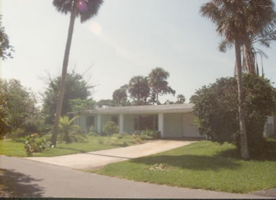
The monitored building is a single family detached structure with a total floor area of approximately 1,795 square feet. However the attached Florida room (300 square feet) and garage (200 square feet) are not conditioned. The conditioned floor area is approximately 1,300 square feet. Figure 1 illustrates the residence's general configuration and orientation. The house faces north-south and is located two blocks from the Atlantic Ocean in Cocoa Beach, Florida.
The floor
consists of slab on grade construction without carpeting (terrazzo).
Built in 1958, the walls are typical concrete block construction with
no insulation. However, approximately ten inches of fiberglass insulation
has been blown into the attic. The attic space is ventilated by soffit
vents and two roof-top rotary ventilators. The attic space is open
to the garage space which does not have a ceiling and is open directly
to the roof decking. The house is fairly well shaded by a tree on
the east face; an outdoor swimming pool is situated on the south side
of the building.
Audit
The house was audited at the beginning of the study according to an established protocol for existing residential buildings (Ternes, 1987). The audit examines all the characteristics of the building that may be related to energy use along with the contained equipment which uses electricity or other fuels. The completed audit instrument is contain in the report as Appendix A.
A series of tests were also completed to establish the air tightness of the structure, before and after duct leakage repair. This consisted of blower door fan-pressurization tests and sulfur hexafluoride (SF6) tracer gas tests to determine the house air infiltration characteristics. The later test was completed, both with the house only exposed to local weather as well as with the air handler powered. The infiltration test results are describe in Table 1:
| Table 1 | |
|---|---|
| Infiltration Tests of the Monitored House | |
Test |
Test
Result |
Blower
Door Air Change Rate |
9.3
ACH |
@50
Pa |
|
%
of Leakage in Duct |
18.2% |
Tracer
Gas Tests |
|
Natural Air Infiltration |
0.58
ACH |
Air Handler Operating |
0.86
ACH |
Return Leak Fraction |
9.7
% |
One year of utility data was collected for the home. Figure 2 illustrates the monthly electricity consumption which totalled 9,774 kWh from April, 1990 through March, 1991. The data clearly shows increased electrical consumption associated with air conditioning in the months of July - September. The base load, including hot water use appears to be only about 600 kWh per month.
Space Conditioning Equipment
The space conditioning system consists of an aging 2.0 ton Sears Climate Master air-to-water heat pump. The air conditioner and air handler are located in the west-facing single-car garage.
The
air distribution system consist of approximately sixty feet of
R-5 rigid-fiberglass ducts which pass through the unconditioned
attic. A total of seven supply registers provide conditioned air
to the house interior. However, only a single ten foot air return
is available from the kitchen area. The measured air handler fan
flow rate was 1,270 cubic feet per minute.
The relative performance of the cooling system is poor compared to
newer more efficient units. Maximum compressor current draw at 240
volts is approximately 19 amps. The measured cooling capacity under
minimum capacity conditions (67.4 °F. dry bulb) was 20,884 Btu/hr
corresponding to an energy efficiency ratio (EER) of 5.2 Btu/W. The
measured before and after coil enthalpy showed a 18 °F temperature
drop across the evaporator when in cooling mode under normal summer
conditions. Capacity at a 88 °F outside temperature was measured
at 28,478 Btu/hr or an EER of 6.5 Btu/W.
A four day test of the air conditioner thermostat performance was performed by Hugh Henderson beginning on July 16th with a separate data logger to characterize its operation. The tests revealed an average air conditioner run-time of 27.0% and an average interior relative humidity of 60.0%. The average thermostat dead-band was quite large at 4.67 °F. The thermostat exhibited the customary degree of thermostat "droop." This provides lower interior temperatures and relative humidity during periods of considerable hourly air conditioner cycling. Equations were regressed from the collected data which showed the average interior temperature and relative humidities to be well characterized by:
Tavg = 77.76 + 3.18 (RTF)
RHavg = 58.82 + 3.23 (RTF)
Where:
RTF = run-time fraction
Instrumentation
The installed instrumentation consisted of a total of eighteen measurements considered important to answer the established research questions. Site weather data is gathered on temperatures, relative humidity, wind speed and insolation. Temperature, humidity and power consumption measurements are taken on the interior of the building. Table 2 lists the measurements taken in the study.
| Table 2 |
|---|
| Monitoring Data Set |
Temperature |
1.
Outside air temperature 2. Interior main zone air temperature 3. Kitchen air temperature 4. Supply register temperature 5. Slab floor temperature 6. Attic air temperature 7. Garage temperature 8. Refrigerator fresh food compartment temperature 9. Freezer compartment temperature 10. Ground temperature (1 ft depth) 11. Pool temperature (2.5 ft depth) |
Single-ended
voltage measurements |
1.
Pyranometer (rooftop) 2. Ambient Relative humidity 3. Interior Relative humidity |
Pulse
Counts Measurements |
1.
Wind speed (10 ft height) 2. Air Conditioning/Heat Pump/Strip Heat Watt-hours 3. Refrigerator Watt-hours 4. Refrigerator Door Opening |
Type-T copper-constantan thermocouples are used to record air and surface temperatures. Measurements of pool water and earth temperature were made using double-ended thermocouples due to potential grounding problems. Single-ended thermocouples were used for all other measurements. Humidity is measured using bulk-polymer resistive type hygrometers. Insolation is measured using a silicon-cell pyranometer with a current output; wind speed is measured with a cupped anemometer which provides pulses to the data logger. Electrical consumption is recorded using two 30 amp pulse-initiating power meters.
All instrumentation was calibrated according to established procedures (see Hurley, 1983). When possible most instruments were calibrated on site. Thermocouples were calibrated at three temperatures (32 °F, 75 °F and 130 °F) with NIST traceable thermometers. The two hygrometers were compared to a General Eastern chilled mirror hygrometer which yield corrections (offset and multiplier) for both instruments. The installed pyranometer was compared to clear day readings from an on-site Eppley PSP. The two power meters were calibrated using a Magtrol 4260 Power Analyzer. The wind speed measurement has been compared to a hand-held anemometer on a portable Solomat instrument to insure consistency.
Data Collection and Acquisition
A Campbell C21X data logger provides the data collection for the research effort. A total of eighteen channels of data is recorded. All the installed instruments are scanned every five seconds with integrated averages and totals output to final storage every fifteen minutes. The technical characteristics of the data logger is included as Appendix B. The data logger holds 29,000 data values in its volatile memory. With twenty data values stored four times an hour the data logger can store approximately eight days of data before retrieval is necessary. The data has been removed periodically using an on-site IBM personal computer with a direct link to the data logger. The data is then read into a statistical analysis package for plotting and later analysis.
With nine months of data collected so far the data retrieval success rate has been 99.3% with only two days of data lost throughout the entire period. The only other data corruption has occurred from the occasional grounding on some of the single-ended thermocouples yielding erroneous results.
These problems have been traced to water condensation of the tip of the thermocouple lead in the refrigerator freezer compartment and electrical grounding problems for the house wiring which provides power to the data logger. Use of a double-ended thermocouple measurement would end the potential problems with the temperature measurements. The grounding problem was solved by installing an earth grounding rod and then tying the house ground to the rod at the electrical panel.
Standardization of Reporting Format
Based on a number of recommendations (Mazzuchi, 1986; Harrje, 1986) a daily examination of recorded data was deemed necessary. This process includes pre-programmed automated data handling with error detection on the data set. All data provided by the data logger is already translated into appropriate engineering units and archived in an ASCII format. Errors are readily detected by the use of DOS batch files on an IBM PC computer which provides initial range checks for reasonableness of all data before it is formatted for plotting. Data which was out of range is then noted and replaced with missing values in the compressed format record.
The data is plotted automatically using available software. Figure 3 shows an example plot of the daily site conditions. Figure 4 shows an example of the plot of air conditioner electrical demand. The data clearly shows air conditioner cycling with the unit turned off at 9:30 AM. Figure 5 shows how the previous two plots can be combined into a single graphic including data showing internal temperature and humidity conditions. Thus, with adequate planning, a single graph for each site automatically produced at midnight provides all the information necessary for the analyst to easily evaluate the success of data collection at a particular site on the following morning.
Air Conditioning Load Shape
One of the stated objectives of this pilot project was to develop an air conditioning load shape profile. Figure 6 shows the air conditioning electrical load over the entire summer. The season begins around julian data 182 (July 1st) and continues through the end of August. Unfortunately the thermostat transformer failed in early September while the occupants were on vacation. Figure 7 shows a box plot of the air conditioner electric power demand for each hour over the entire summer while the system was properly functioning. The box plot shows that the air conditioner electric power demand is less than a thousand watts in the early morning hours and does not vary substantially from one day the next (the compact length of the boxes). However, the building air conditioning load clearly picks up at 11 AM reaching a peak at the 5 - 6 PM hour with a median demand of nearly 2,500 watts. It is also noteworthy that demand on any given day during the peak hours is quite variable with the outer quartile ranges stretching from 400 - 4,500 watts. The shape of the described profile agrees well with utility metering of the air conditioning demand of a number of homes in the Florida Power and Light service territory (Paxson and Hinchcliffe, 1980).
Analysis of Savings from Duct Repair
The second objective of the monitoring was to ascertain the effect of duct repair on the house air conditioning demand. The experiment began in July. Two weeks of 15-minute data were collected with the air conditioner and duct system in an "as is" configuration.
After this time the air conditioner was serviced by Atlantic Air on August 1st. Unfortunately, the service personnel repaired major return side duct leaks at the time of the service. Realizing the dilemma that this caused, a one square inch of duct leakage was re-opened at the old duct leak site. It appears, however, that the area repaired by the service person was considerably larger than the one created.
After another three weeks the duct system was sealed with mastic by Natural Florida Retrofit on August 27th. Blower door testing before and after the duct repair showed that 71% of the measured duct leakage area was sealed. The air conditioning consumption was then monitored for another two weeks. Unfortunately, one week of this data was lost when a transformer failed which powered the air conditioner. Unfortunately, the problem was not corrected until the investigator returned from vacation after which the cooling season was over.
The duct repair did show major savings in air conditioning energy use. It is not possible to estimate savings due to the air conditioner service since duct leaks were sealed at the same time. In general, the duct repairs reduced air conditioning use by about 19% for a group of days with similar interior-exterior temperature differences. This result compares favorably with the 17.2% savings realized in 46 homes with duct system which were repaired (Cummings et al., 1991). The data collected for the single house is summarized in Table 1:
|
Table
3 |
||||
|---|---|---|---|---|
Daily
Air Conditioning Electrical Consumption Before and After Duct System Repair |
||||
Case |
No.
Days |
kWh/Day |
Std.
Devn. |
dT
(°F) |
Before
Repair |
6 |
45.50 |
13.01 |
5.15 |
After
Repair |
4 |
36.74 |
1.94 |
5.83 |
Difference |
8.76
(19.3% Reduction) |
|||
Reductions to Time-of-Day Electrical Demand
Figure 8 shows the hourly monitored cooling energy use before and after duct system repair. In the upper panel, the hourly electrical demand is plotted against the interior to garage temperature difference. The lower panel compares the same air conditioning electrical demand data to the inside to ambient temperature difference. Examination of the two plots reveals that the garage temperature conditions are much more strongly related to the air conditioner loads. Air conditioning demand is more weakly linked to ambient to interior temperature differences. Regression lines predict that for a given degree of temperature difference between the interior and the garage, the air conditioner will use 24% less electricity after the duct repair.
Figure 9 shows the monitored electrical demand of the air conditioner on the two hottest pre and post repair days. The pre-repair day was July 31st and the post-repair day was August 31st. The electrical demand in watts for a running 60-minute average is plotted for both days. Total daily electrical consumption is 58.4 kWh before duct repair and 34.2 kWh after-- a total daily savings of 41%. The ambient temperature conditions present during the two days are compared in the lower panel.
The graph illustrates the large magnitude of the potential savings during hot afternoons which may be available from sealing duct leakage. Prior to repair, the air conditioner runs constantly from 3 P.M. to 8 P.M. with an average electrical demand of 4,525 Watts. After the duct repair the capacity of the machine is never reached and average electrical demand during the same period on August 31st averages only 2,338 Watts. Thus, the avoided peak period electrical demand is nearly 2.2 kW. The non-peak period electrical demand was 1,835 Watts before duct repair and 1,172 Watts after. The savings during the non-peak period are fractionally large (36% of pre-repair consumption), but small in magnitude (663 Watts). The results indicate that electrical savings from duct repair are strongly machine run-time dependent.
In summary, analysis reveals the following:
● Daily air conditioning energy savings from duct repair averaged about 20% for a group of days with similar temperature differences.
● Savings are strongly time dependent. Figure 9 shows that duct repair resulted in over a 2 kW electrical load reduction on the two hottest days available for the analysis. Daily energy consumption was 39% lower after duct system repair for these days. Analysis indicates the weather on the two days was roughly comparable.
● The air conditioning electrical demand is best correlated with the interior to garage temperature difference. The air handler is located in the garage in the monitored house which controls the temperature and enthalpy conditions of much of the return leaks to the system. This finding may have large implications for the effects of air handler location on air conditioner efficiency in Florida homes. Given this result, one would expect that air handlers located in attic spaces (fairly common in the state) will exhibit even worse performance due to the very high temperature conditions present.
It is commonly assumed that residential refrigerators possess a relatively flat load shape in an air conditioned house. Monitoring of the refrigerator-freezer in the pilot study revealed otherwise.
There are approximately five million residential refrigerators in Florida. The average demand of these units is at least 1,000 MW. The least efficient refrigerators are existing models of which approximately 5% of the stock is replaced each year. The average life expectancy of a residential refrigerator is 20 years (ACEEE, 1990) such that at least 25% of Florida's existing stock are old inefficient units. Replacement of these units represents a very significant opportunity for utility demand side management.
The existing refrigerator, which has been in service for approximately 15 years, is similar to many other models of its type which are soon to be replaced. The unit is a 19.2 cubic foot frost-free Sears Coldspot refrigerator-freezer with an automatic ice maker and a water dispenser. Monitoring has shown its summertime utility peak hour (5 - 6 PM) electrical demand to average approximately 303 W with annual consumption of about 2,510 kWh-- a very substantial end-use of electricity in the home. Based on monthly utility bills from the monitored house, the refrigerator represents over 25% of the total annual electrical use in the home. Table 4 summarizes the data taken on the refrigerator performance:
| Table 4 | ||||
|---|---|---|---|---|
| Refrigerator Performance | ||||
Value |
Mean |
Std.
Devn. |
Min |
Max |
Main
Food Temp (°F) |
38.3 |
3.36 |
31.9 |
55.7 |
Freezer
Temp (°F) |
07.7 |
4.35 |
-1.6 |
44.4 |
Kitchen
Temp (°F) |
84.1 |
3.49 |
78.5 |
94.2 |
Electrical
Demand (W) |
287.3 |
60.4 |
22.5 |
446.5 |
Electrical
Demand (W) |
||||
2 - 8 PM |
307.5 |
64.0 |
22.5 |
446.5 |
5 - 6 PM |
303.3 |
63.4 |
167.4 |
446.4 |
This estimate is in line with another monitoring study in Florida which found an average household electrical use of 3,734 kWh for refrigeration including households with separate freezers and second refrigerators. The average annual use for each monitored refrigerator-freezer was 2,361 kWh (Messenger et al., 1982). Refrigeration in that study accounted for 15.1% of overall residential electrical consumption.
The existing refrigerator will be monitored for one complete year to obtain time-of-day demand for each season. This will give an indication of the magnitude of peak and annual electrical demand from older existing refrigerator stock in Florida houses.
In July, 1991, he existing refrigerator will be replaced with the most energy efficient model in its size and type possessing the consumer desirable amenities (automatic ice-maker, automatic defrost) (ACEEE, 1990). Before and after 15-minute electrical demand will be obtained and compared in a future research report.
Figure
10 shows an example of data collected from the refrigerator over
a five day period in August. The freezer compartment temperature
clearly show the periodic defrost cycles of the unit. Heavy use
of the unit on August 11th during a dinner party is clearly evident
(and a good illustration of the need for occupant reported events
that may influence energy use). Figure 11 depicts the raw electrical
demand of the refrigerator over the month of June. Even with the
great amount of scatter, some daily trend is evident. Figure 12
shows the data for the entire summer interpreted as a series of
box plots. The display shows a definite time-of-day use pattern
for the refrigerator; electrical demand is highest at 8 PM subsequent
to dinner preparation.
Attic and Garage Temperatures
Data analysis of the air conditioning load revealed that the interior to garage temperature difference was much better at predicting air conditioner electrical use than was the temperature difference to ambient conditions. Figure 13 shows the electrical demand on July 31st, prior to duct repair, superimposed against both inside-to-ambient and inside-to-garage temperature differences. Presumably, this phenomenon is caused by the importance of the temperature and humidity conditions of the source of return air leaks around the air handler unit. Another factor may be the heat gain to the air handler housing itself.
The data shows that in the studied house, where the air conditioner is located in the garage, its electrical demand is much more closely linked to garage temperatures than ambient conditions. The data illustrates the importance of the thermal conditions in buffer spaces in determining air conditioning electrical demand when there is substantial return side leakage which may be linked to these spaces.
Figures 14 and 15 show that the summertime temperatures in the garage and attic spaces in the monitored home are quite high. The summer garage temperatures are almost always higher than the ambient daily temperature-- commonly reaching over 90 °F. The difference between the garage and ambient temperature is most pronounced during the afternoon peak load hours. The rapid drop in garage temperature on the final day shown is due to a sudden afternoon rain storm. Attic temperatures are even greater, as shown in Figure 15. Peak temperatures may reach nearly 120 °F although the attic cools off rapidly during the evening hours, often to a level lower than the ambient temperature due to the radiative cooling of the roof surface to the night sky. Figure 16 summarizes the average 15-minute garage, attic and ambient air temperatures for the month of July while the house was almost continuously air conditioned.
Table 5 summarizes the four summer months of data on the garage and attic temperatures in the home and also provides a summary of these temperatures during the utility peak demand hour. This data shows that the average attic and garage temperatures from 5 - 6 PM is over 90 °F:
| Table 5 | ||||
|---|---|---|---|---|
| Garage and Attic Temperatures | ||||
Value |
Mean |
Std.
Devn. |
Min |
Max |
Garage
Temp. (°F) |
88.1 |
4.5 |
76.2 |
99.8 |
Attic
Temp. (°F) |
87.6 |
10.1 |
72.1 |
119.1 |
Ambient
Temp. (°F) |
84.5 |
5.3 |
72.1 |
98.6 |
5
- 6 PM |
||||
Garage
Temp. (°F) |
||||
Attic
Temp. (°F) |
||||
Ambient
Temp. (°F) |
86.0 |
4.9 |
73.7 |
93.6 |
Floor Slab Cooling Potential
Like most Florida homes, the studied house has a slab on grade foundation. However, the monitored house is somewhat unique in that the floor is not carpeted and has a terrazzo surface. Previous research has indicated that exposed floor slabs may offer some cooling season benefit for Florida homes (Fairey et al., 1986).
Figure 17 gives an indication of the moderating influence of the ground as a heat-sink during periods of natural ventilation. The ground temperature at a 2.5 foot depth varies only slightly over the daily cycle over the entire summer in contrast to the large amplitude of the swing in daily air temperature. Figure 18 shows the distribution of living room and floor slab temperatures over a hot week-long period in June when natural ventilation was utilized. The daily cycle of heat storage within the floor slab is quite obvious in the plot. This indicates that the slab mass is providing a significant moderating influence on the house internal temperatures when ventilating. Figure 19 shows the slab temperature against the main zone temperature for the entire summer period. It is noteworthy that the slab temperature is lower, even during periods of air conditioning.
Table 6 summarizes the data on the floor slab and main zone (living room) temperature, both while naturally ventilating and when air conditioning. The data shows that the floor slab surface is cooler under both conditions. Assuming a 1,000 square feet of exposed terrazzo and use of the ASHRAE surface heat transfer coefficient (1.08 Btu/hr⋅ft2⋅°F) the data indicates an average level of cooling from the slab of approximately 1,500 Btu/hour when ventilating and half this figure when air conditioning at an average 81 °F interior temperature. It appears likely that a floor slab is adiabatic for cooling set points between 77 and 80 °F.
| Table 6 | ||||
|---|---|---|---|---|
| Main Zone and Floor Slab Temperatures | ||||
Value |
Mean |
Std.
Devn. |
Min |
Max |
Air
Conditioning |
||||
Main
Zone Temp. (°F) |
81.6 |
1.76 |
76.2 |
86.8 |
Slab
Temp. (°F) |
80.9 |
1.23 |
77.6 |
84.4 |
Ventilating |
||||
Main
Zone Temp. (°F) |
85.3 |
3.06 |
78.4 |
92.4 |
Slab
Temp. (°F) |
83.9 |
2.28 |
78.8 |
88.6 |
Effect of Building Mass on Natural Ventilation Potential
The
monitored house has concrete wall construction with a slab on grade
foundation. This is typical for many existing Florida homes. Such
a massive construction should lead to a structure which moderates
the swing in daily internal air temperatures.
Figure 20 shows a plot of the ambient air and living room temperatures
over a five day period in June in which the house was naturally ventilated.
The moderating influence of the building mass is clear; the ambient
temperature both rises higher during the day and, at night, falls
lower, than the internal temperature which varies considerably less.
However, the data also shows that outside nighttime temperatures
are always closer to comfort conditions than the interior conditions
even with windows open. Two important reasons for this nightly difference
are 1) the delayed solar heat flux through the walls of the building
and 2) the very low wind speeds which are typical on hot summer days.
Figure 21 shows the average interior, slab and ambient temperatures for the entire natural ventilation period in June. The data shows that on average the outside air temperature becomes less than the main zone temperature at 3 PM, and that substantial differences exist during the entirety of the evening hours. During this time ambient temperatures are much closer to comfortable levels.
These results indicate that a whole house fan which assisted air flow to the interior at night would provide significant improvements in comfort in high-mass Florida homes during periods when natural ventilation is utilized. Such a strategy would help to rapidly remove the accumulated heat within the building walls while maintaining comfort conditions to an acceptable level. Presumably, such forced ventilation would also extend the morning comfort conditions by storing night "coolth" within the massive construction of the house.
Kitchen Comfort Conditions
Based on the monitoring results, the kitchen is far warmer than the main zone even when the occupants are relying on natural ventilation to reduce air conditioning loads. Figure 22 shows a comparison of the average kitchen and living room zones for the early summer when natural ventilation was used to meet cooling loads. Figure 23 presents a similar plot for a comparison of the main zone and kitchen air temperatures while the house was air conditioned. This plot shows the typically experienced "thermostat droop" where the interior temperature maintained by the thermostat drops as machine run-time increases. The scatter plots shows two trends with which almost every Florida cook will agree:
1) Kitchens are warmer than most other rooms
2) Kitchen temperatures can reach intolerable levels when cooking is taking place.
Table 7 summarizes the data under both natural ventilation and air conditioning periods:
| Table 7 | ||||
|---|---|---|---|---|
| Main Zone and Kitchen Temperatures | ||||
Value |
Mean |
Std.
Devn. |
Min |
Max |
Air
Conditioning |
||||
Main
Zone Temp. (°F) |
84.1 |
1.94 |
78.5 |
94.2 |
Slab
Temp. (°F) |
81.6 |
1.76 |
76.2 |
86.8 |
Ventilating |
||||
Main
Zone Temp. (°F) |
85.8 |
3.25 |
78.4 |
95.4 |
Slab
Temp. (°F) |
85.3 |
3.08 |
78.4 |
92.4 |
Such data suggests that use of whole house fans which exhaust from the kitchen area or vent fans which would be activated by range top operation would provide substantial relief to house comfort during the swing seasons when little air conditioning is otherwise needed.
Effect of Suspension of Air Conditioning on Interior Humidity Levels
A commonly posed question for the feasibility of thermal storage systems to provide adequate comfort in cooling dominated climates has to do with how much moisture interior furnishings in houses can absorb before humidities reach uncomfortable levels. This is important since DSM strategies which involve sudden cessation of mechanical air conditioning during peak load hours may lead to excessive interior moisture levels (and temperatures) within a short period of time.
Figure 24 shows an experiment that was performed on July 21st, a hot summer day. At 9:30 AM the air conditioner was turned off, but the building was left closed until 5 PM. The data shows that the humidity level increased rapidly until roughly 1 PM, but then reached a plateau around 67% where it remained until suddenly increasing when the windows were opened. The data indicates that a substantial amount of moisture may have been absorbed by the interior furnishings. Unfortunately, the data also shows that the interior air temperature left the comfort range within an hour of mechanical cooling being shut off. Further experiments of this type are desirable for the next cooling season.
Influences on Swimming Pool Temperature
The swimming pool temperature was monitored at a 2.5 foot depth over the monitoring period. The pool is kidney-shaped with a capacity of approximately 15,000 gallons. The pool is not covered by a screen and no shading is present. An insulating pool cover is not used. Figure 25 shows a plot of the pool temperature compared with the 2.5 ft ground temperature over the entirety of the summer. The plot shows a much greater daily variation in the pool temperature than that of the ground with a pronounced daily cycle. Examination of the individual daily plots reveals that the pool reacts almost immediately to available solar flux on a given day as shown for the three days of varying solar radiation in Figure 26. Subsequent analysis of the weather data reveals that a number of factors affect the changing pool temperature over the course of the season. Wind speed and humidity (convective heat transfer and evaporation) appear to be large influences as are the solar flux and air and ground temperatures. A relatively simple multiple regression model predicts 81% of the hourly variation in measured pool temperature over the entire summer:
Where
pool
= pool temperature in the next hour (F.)
tamb = ambient air temperature (F.)
solar= the solar insolation (W/m2)
ws = wind speed (mph)
tgrd= measured ground temperature at 2.5 ft depth (F.)
ambrh = measured outdoor relative humidity (%)
evap = (100- ambrh) * ws
night = dummy variable for nighttime hours (9 PM - 5 AM)
convec = (tpool - tamb) * wind speed
esky = (100 - RH) * night
Recommendations for Existing Florida Homes
The following recommendations for improving the energy efficiency of existing Florida homes can be made based upon the monitored data for this single building. The success of this initial effort indicates the relative efficiency of even single case studies to provide practical design information.
● Repair of duct leakage for air conditioning systems appears quite beneficial to reduction of cooling electrical use. Air conditioning loads were reduced by
approximately 19%.● Air handler location and associated enthalpy conditions may have very large impacts on the relative efficiency of residential space cooling systems. Analysis of the monitored system, which has a garage located air handler, revealed that the air conditioner electrical consumption was strongly influenced by the garage temperature conditions, even after duct leakage repair. The garage temperature was also found to be consistently higher than that ambient temperature throughout the air conditioning season.
● Retrofit of old inefficient refrigerators may offer a significant savings potential in existing Florida homes. The monitored unit will use an estimated 2,500 kW annually (over 25% of the total annual consumption in the studied house) and contributes 0.30 kW to the summertime peak coincident electrical demand.
● Nighttime use of whole house fans appears to offer significant potential to enhance comfort conditions when natural ventilation is utilized in Florida houses.
● Ventilation of Florida homes using whole house fans will do best to draw
air from the warm kitchen area.
Lessons Learned
The following represents a list of lessons learned from the pilot study with respect to future larger-scale monitoring projects:
● Research depth with simplified monitoring protocols (few data points, low level data collection) can be significantly enhanced by the use of a few case-studies of buildings with more detailed monitoring which are embedded within a study.
● Daily data collection and plots are advisable to insure data consistency and quality.
● An expert system to check the validity of incoming data is an important aspect to a successful data acquisition system.
● An occupant activity log which reports significant lifestyle changes, vacations etc.
can be useful to assist in later data interpretation.● Double-ended thermocouples are preferable for locations where grounding or excessive moisture may occur.
● The utilized data logger was quite reliable although special care must be provided to ensure that a true earth ground is available for the power source.
Future Monitoring and Experimentation
The house will be monitored for air conditioning loads again this summer. Since only four days of useful post-repair data was obtained last summer, monitoring this cooling season will emphasize obtaining more data on performance after the repair. This will also allow examination of the persistence of the savings from the duct leakage repair.
The existing refrigerator will be monitored through June, providing a full year of data on this existing model. At the end of the month the unit will be changed out to the most efficient model within the same size class. The new refrigerator will then be monitored over the following year. This monitoring will provide unique data on the savings of existing refrigerator retrofit and the load shape of the available savings. This data will be presented as a monitored example of a potential demand side management strategy for utilities.
A series of other possibilities for future experimentation with the house are briefly outlined below:
● Influence of the use of a pool cover on the length of the pool swimming season.
● Whole house fan enhancement in comfort conditions during natural ventilation.
● Reduction in attic temperatures achieved by: a) use of rotary roof-top ventilators and b) roof covering with a white elastomeric coating.
● Further experiments on moisture absorption inside the house when mechanical cooling is temporarily suspended.
● "Flip-flop" tests of the alternate substitution of compact florescent lighting with conventional bulbs on the appliance electrical demand.
References
ACEEE, 1990. "The Most Energy-Efficient Appliances: 1990 - 1991 Edition, American Council for an Energy Efficient Economy, Washington D.C.
J.B. Cummings, J.J. Tooley and N. Moyer, 1991. Investigation of Air Distribution System Leakage and Its Impact in Central Florida Homes, Florida Solar Energy Center, FSEC-CR-397-91, Cape Canaveral, FL.
P. Fairey, A. Kerestecioglu, R. Vieira, M. Swami, S. Chandra, 1986. Latent and Sensible Load Distributions in Conventional and Energy Efficient Residences, prepared for the Gas Research Institute, Florida Solar Energy Center, FSEC-CR-153-86, Cape Canaveral, FL.
D.T. Harrje, 1986. "Obtaining Building Energy Data-- Problems and Solutions," Proceedings of the National Workshop on Field Data Acquisition for Building and Equipment Energy Use Monitoring, Oak Ridge National Laboratories, prepared for U.S. DOE, DOE CONF-8510218, Dallas, TX.
C.W.
Hurley, 1986. "Measurement of Temperature, Humidity and Fluid
Flow," Proceedings of the National Workshop on Field Data
Acquisition for Building and Equipment Energy Use Monitoring, Oak
Ridge National Laboratories, prepared for U.S. DOE,
DOE CONF-8510218, Dallas, TX.
M. D.
Lyberg and G.V. Fracastoro, 1986. "An Overview of the Guiding
Principals Concerning Design of Experiments, Instrumentation and
Measuring Techniques," Proceedings of the National Workshop
on Field Data Acquisition for Building and Equipment Energy Use
Monitoring, Oak Ridge National Laboratories, prepared for U.S.
DOE,
DOE CONF-8510218, Dallas, TX.
R.P.
Mazzucchi, 1986. "Design of a Large Scale Metering Project," Proceedings
of the National Workshop on Field Data Acquisition for Building
and Equipment Energy Use Monitoring, Oak Ridge National Laboratories,
prepared for U.S. DOE,
DOE CONF-8510218, Dallas, TX.
R. Messenger et al., 1982. "Maximally Cost Effective Residential Retrofit Demonstration Program," prepared for the Florida Public Service Commission, Florida Atlantic University, Boca Raton, FL.
D.F. Paxson and G.R. Hinchcliffe, 1980. Residential Air Conditioning Load Study, Florida Power and Light Company, Energy Management Research Department, Miami, FL.
M.P.
Ternes, 1987. "Single Family Building Retrofit Performance
Monitoring Protocol: Data Specification Guideline," Oak Ridge
National Laboratory, ORNL/CON-196,
Oak Ridge, TN.
© 2007-2014 University of Central Florida. The Florida Solar Energy Center (FSEC)
is a research institute of the
University of Central Florida.
For more information about FSEC, please contact us or learn more about us.
Find us on Facebook!