

Reference Publication: Fairey, P., D.S. Parker, B. Wilcox and M. Lombardi, "Climate Impacts on Heating Seasonal Performance Factor (HSPF) and Seasonal Energy Efficiency Ratio (SEER) for Air Source Heat Pumps." ASHRAE Transactions, American Society of Heating, Refrigerating and Air Conditioning Engineers, Inc., Atlanta, GA, June 2004. Disclaimer: The views and opinions expressed in this article are solely those of the authors and are not intended to represent the views and opinions of the Florida Solar Energy Center. |
Climate
Impacts on Heating Seasonal Performance
Factor (HSPF) and Seasonal Energy Efficiency
Ratio (SEER) for Air Source Heat Pumps
Philip
Fairey1, Danny Parker1, Bruce
Wilcox2 and Mathew Lombardi1
1Florida
Solar Energy Center (FSEC)
2Berkeley Solar Group, Berkeley, California
FSEC-PF-413-04
Abstract
Within rating procedures established by the U.S. Department of Energy, benchmarks have been established for the comparative performance of heat pumps and air conditioners. The Heating Seasonal Performance Factor (HSPF) and Seasonal Energy Efficiency Ratio (SEER) index heating and cooling season performance, respectively. Although the procedures result in a highly desirable standard metric, the climate related limitations of the published values must be understood – particularly when attempting to extend performance prediction across regions. This paper describes evaluation of climate related variation of heat pump and air conditioner performance. Operating seasonal efficiencies are statistically related to location specific winter and summer design temperatures and manufacturers’ equipment ratings. Implications are discussed.
Heat Pumps
Residential air source heat pumps are an increasingly popular heating system in the southern United States. Over 10 million heat pumps (HPs) are currently in use (EIA, 2001). The practical efficiency that air-source heat pumps achieve is a coefficient of performance (COP) of 2.0-3.0. To rate heat pumps in a standard fashion, a Heating Seasonal Performance Factor (HSPF) is determined which takes into account operation under varying outdoor temperatures as well as part load impacts (effects of running short cycles under mild conditions). HSPF is rendered as Btu/Watt-hour so that typical HSPF are nominally on the order of 6.8 - 10 Btu/Wh (the dimensionless value of the minimum HSPF of 6.8 is COP = 1.99). HSPF is defined according to test procedures as promulgated by ARI in its Standard 210/240 as well as ASHRAE Standard 116 and the DOE Test Procedure in 10 CFR; Part 430, Appendix M (ARI, 2003).
The rated/nameplate HSPF from ARI 210/240 is based on the temperature in Climate Region IV (2000-2500 heating load hours) and the minimum Design Heating Requirement (DHR) that is a function of machine heating capacity. This selection is favorable to limit the contribution of resistance heating because it typically results in a balance point in the 17 to 25EF range. Although published HSPFs are linked to this climate, and specifically to 2080 heating load hours, it was never envisioned that this single value could be used to generically predict performance for all climate locations. Given the severity of winter in much of the continental United States and the sensitivity of heat pumps to the outdoor temperature, site specific performance must vary significantly with climate. Although temperature bin data and procedures within ARI 210/240 are available to compute performance in other climate regions (Sections A.6.2.4 and A.6.2.5 of that standard), the published data available for all heat pump and air conditioning units is that of Climate Zone IV. Thus, although a method is available to compute HSPF and SEER in other regions, this is not done and the information is unavailable to consumers and others without access to data on machine performance at the specific test points.
The ARI directory of Certified Unitary Air-Source Heat Pumps does provide rudimentary information on heating performance for all six heating regions. The directory includes a table entitled "Heating Cost Factor" which provides information, which can be used to adjust the annual energy cost based on the FTC-labeled amount for Region IV for each unit that is listed to annual energy costs for the other five regions. Unfortunately, as will be shown within the paper, the climate classifications within the ARI directory’s map leave much to be desired relative to accuracy in capturing winter severity. Also, the methods used to estimate the heating system performance within the procedure itself tends to be optimistic relative to typical operating conditions, setpoints etc.
Moreover, the six climate zones available within the ARI 210/240 method are necessarily coarse with respect to climate. For instance ARI Climate Zone 2 includes the widely varying climates of Phoenix (1125 Heating Degree Days (HDD)/4189 Cooling Degree Days (CDD), 99% Design Temp=37ºF, 1% Design Temp=108ºF) and Ft. Worth, Texas (2370 HDD/ 2568 CDD, 99% Design Temp=24ºF, 1% Design Temp=98ºF).
Although it was never intended that the Region IV HSPF and SEER would be used to estimate energy use across climates, these values have indeed been used for these purposes within software and calculation procedures (for instance see Manual J, 7th Edition, Appendix A-4 "Energy Consumption and Operating Cost", ACCA, 1986). Particularly, for heat pumps, this can lead to erroneous conclusions on their relative merit as compared with non-heat pump alternatives across climates. Given these limitations, it is highly desirable to have some means to interpret the seasonal performance of heat pumps and air conditioners across locations.
Beyond the climatic variation, there are other reasons that typical performance may not reach that suggested by the ARI standard. Within the 210/240 procedures, a correction factor, "C” with a value of 0.77, is used to reduce the heating loads on the heat pump. The justification for the C factor is that it more closely matches measured building loads when used with degree day or bin weather data based on a 65oF set point (Harris et al., 1965). The reason the building loads are lower is due to heat gains, such as solar gains and internal gains, which cause a balance point lower than 65oF. A better method to account for this is to use a lower balance point, rather than a multiplier, since the effect at varying outdoor temperatures can be very different than the C=0.77 default. For instance, tests performed by the Electric Power Research Institute in the late 1970s found that "C" could vary from 1.2 to 0.4 in actual residences (EPRI, 1980). As a result, the method of estimation has fallen out of favor as evidenced by its disappearance from the ASHRAE Handbook of Fundamentals after 1985.
Another associated problem with the ARI procedure is that it implicitly assumes a 65oF interior heating setpoint by using bin data at 65oF along with "C" to reduce those loads. In our analysis we desired to use the more commonly preferred 68ºF interior heating setpoint. This will have the effect of increasing the building load, which in turn will tend to reduce the simulated HSPF as compared with the assumption of 65oF as in ARI 210/240. Backup resistance use will also increase. At an outdoor temperature of 45ºF, this difference could impose a 30% increase in loads after internal and solar gains are taken into account.
Cooling Mode Operation and SEER
The seasonal energy efficiency ratio (SEER) rating for central air conditioners was adopted in 1979 after years of development. Last modified in 1994, SEER is a national metric that does not account for regional differences in summer climate. In addition, the SEER rating de-emphasizes high temperature performance (EER95). Indeed, for single-speed equipment the test is entirely based on performance at 82ºF, so designs can be (and often are) optimized for moderate temperatures. Even for modulating equipment, the weight assigned to high temperature performance is very low. Since high temperature performance can vary significantly among designs with the same SEER, and since high temperature performance is a key determinant of utility peak loads, this limitation is of concern. In addition, the ARI standard specifies static pressures that are about half as large as the averages from field studies (Proctor and Parker, 2000). High static pressure means lower air flow across the evaporator coil, which leads to a relatively cold coil, which increases cooling energy use in dryer climates and lowers heat pump performance everywhere.
Similarly, the ARI procedure implicitly assumes an 80ºF interior setpoint for cooling as opposed to the 78ºF setpoint assumed in this study. The more realistic, but lower setpoint will also result in greater loads for the “operating efficiency” calculations performed here and hence result in lower predicted cooling performance. These limitations of the assumptions used within the SEER procedure have been pointed out by others (Kavanaugh, 2002).
When used in cooling mode, the performance of a heat pump is greater due to the smaller temperature differences between indoor and outdoor conditions and the fact that heat is being extracted from the interior of the home rather than from a very cold exterior condition. Thus, typical cooling system SEERs are on the order of 10 - 17 Btu/Wh for current generation equipment. For the analysis presented here, systems with SEERs equal to or greater than 13.5 Btu/Wh are assumed to have electronically commutated motors (ECM) in use within the indoor blower units. Likewise, the analysis assumes that ECMs are utilized where HSPF is equal to or greater than 8.5.
Empirical Tests of Heat Pump Performance
As heat pump technology emerged in the early 1970s, a number of measurements were made on heating system performance. Many laboratory studies were performed under steady state conditions to evaluate the impacts of defrost cycles, crankcase heat and other influences (eg. Parken et al., 1977; Rettberg, 1980). It has been long known that, even with a constant thermostat setting, when building loads exceed the declining capacity of the heat pump, the difference must be made up with resistance heat. This will impact overall efficiency (Reedy and Daniels, 1992).
Many of the existing early studies did show that heat pump performance was often lower than would be expected by the ARI procedures. In a study for Louisiana Power and Light Company, Orth et.al. (1976) performed alternate day resistance heating measurements on two 1967 vintage heat pumps and found seasonal coefficient of performance (SCOP) measurements of 1.75 and 1.78 for the systems as compared with the manufacturer’s SCOP rating of 2.25. In the colder climate of New Jersey, Nicolich (1977) estimated the SCOP of a single heat pump to be 1.65 based on pre and post measurements. In the much colder climate of Ontario, Canada, 40 heat pumps were monitored in detail showing average SCOPs of 1.43 over the heating season from 1975-1977. Similarly, a large study by Carrier Corporation (Groff et al., 1978) showed average seasonal COP values of 1.61 to 1.2 in the Boston and Minneapolis climates, respectively.
However, even in moderate climates, performance may be less than anticipated. Four residences in Albuquerque, New Mexico that had the heating system performance of their heat pumps evaluated through alternate day resistance heat operation showed SCOPs averaging only 1.39 (1.42, 1.10, 1.64 and 1.41) as opposed to the HSPF calculation, which indicated a SCOP of 1.85 (Wildin et al., 1978). Significantly, the study estimated that homeowner operation of thermostats led to lower than expected savings. Another study in Knoxville, Tennessee of two heat pumps (Baxter, 1981) yielded measured SCOPs of 1.58 and 1.99 respectively as compared with labeled SCOPs of 1.99 and 2.61.
Admittedly, the above studies were on early generation heat pumps rather than more modern equipment. However, the relevance of these older investigations is underscored by more recent data suggesting similar trends. Recent sub-metered data from over 160 Florida homes show that operational heat pump performance is adversely impacted by thermostat set back (Bouchelle et al., 1999). This same phenomenon had been observed in earlier research on monitored heat pump performance (Bullock, 1978). Since the utility experiences its annual system peak during Florida’s few cold mornings, the performance of heat pump systems is important to controlling demand. While the mild conditions prevailing should allow heat pumps to operate under favorable conditions, data analysis revealed a large impact from auxiliary electric resistance strip heat on site-achieved heat pump efficiency.
Households practicing temperature setback followed by a morning setup (about 25% of total) showed large amounts of strip heat during morning operation, which reduced overall coefficients of performance (COP). Thus, the measured annual space heat consumption of the 91 heat pump systems was 1,038 kWh as compared to 1,292 kWh for the 57 homes in the electric resistance group. Correcting for differing floor areas, the group of homes with heat pumps showed a normalized energy use of 0.65 kWh/ft2 against 0.94 kWh/ft2 for the homes with electric resistance forced-air heating systems. The implied seasonal COP from these data is only 1.45 compared with the commonly claimed 2.0 (HSPF = 6.8).
Another contemporary source of empirical data on comparative heat pump performance comes from the Pacific Northwest in sub-metered data taken by the Bonneville Power Administration. As part of its Super Good Cents program, hundreds of homes had space heat sub-metered from 1987 - 1991 with detailed audit information on the homes (Andrews et al, 1989; Eckman, 2000).
Within these data, homes in the populous coastal region of the Pacific Northwest showed an average measured annual space heat of 7,841 kWh (3.63 kWh per square foot of floor area) for those with heat pumps (n= 85) against 8,953 kWh (4.46 kWh per square foot) for those with force air electric strip heat (n= 35). Although the savings produced by heat pumps was statistically significant, the implied coefficient of performance was only 1.23 – well below the nameplate COPs of 1.99 or better.
Although not evaluated here, previous monitoring and evaluation has shown that thermostat setback with morning set-up can have very deleterious effects on air-source heat pump performance as the sudden increase in morning thermostat set-up triggers the use of lower efficiency auxiliary resistance strip heat (Bullock, 1978; Bouchelle et al., 2000). These same set-back strategies do not impact resistance heating systems, and thus reduce the relative efficiency advantage of heat pump systems.
Seasonal Energy Efficiency Ratio (SEER)
The air conditioning industry has long relied on SEER as the indicator of central system cooling equipment performance. All unitary air conditioners are rated using EER, a rating standardized by ARI, which reports steady-state efficiency at 95oF outdoor and 80oF indoor temperature. However, these data are not universally reported. Smaller air conditioners (i.e., < 65,000 Btu/h) are also rated using SEER, a rating developed by the U.S. DOE and based on EER, intended to better indicate average seasonal performance, i.e., a season average EER. However, for single-speed equipment, SEER is simply estimated as the EER at test condition “B” which consists of an 82ºF outdoor and 80oF indoor temperature condition.
To obtain SEER, the “B” test condition result is then lowered by a degradation coefficient (CD) to account for cycling losses, which varies depending on fan time delay and refrigerant control strategies. Air conditioning equipment is usually tested for CD, with a median cooling value of about 0.10 for typical units. A default value for CD of 0.25 may be used in lieu of testing, but that option is rarely exercised because of the high default value and the resulting deleterious impact on estimated performance (Doughery, 2003). To obtain higher SEER and HSPF ratings, manufacturers have frequently instituted a timed indoor unit fan off delay and control of post-cycle refrigerant migration to achieve CD values of 0.05 or less.
Given the particulars of ARI test condition “B” SEER is also tied to an assumed 80oF indoor condition – at least two degrees higher than the cooling set point commonly observed in air conditioned residences (Parker, 2002). The current standards mandate air conditioner efficiency levels using EER and SEER and consumers are typically guided to make energy-wise purchases based on these ratings – the higher the SEER, the more efficient the system. Understandably, manufacturers work to improve the SEER ratings of equipment given the current guidelines. Given the current test procedure, there is strong incentive to produce air conditioning equipment that does best under moderate load conditions (see Kavanaugh, 2002).
A recent study by the California Energy Commission has compared SEER data for over 9,600 air conditioners with the EER information on the same units and found that many high SEER units have low high-temperature EERs. Figure 1 is a scatter plot of COP95 (EER/3.413) versus SEER/3.413 for all split system air conditioners in the California Energy Commission (CEC) database. Although there is a general trend there are many high SEER units that have EERs no higher than units with minimum SEER. This is of particular concern in dry climates because the combination of low humidity and high outdoor temperatures mean that air conditioners operate a large fraction of their time at or above the 95ºF outdoor EER rating point. Even more important, however, is the fact that residential air conditioners are a large contributor to peak electrical demand, which occurs during the hottest summer afternoons when the system size and EER determine the demand.
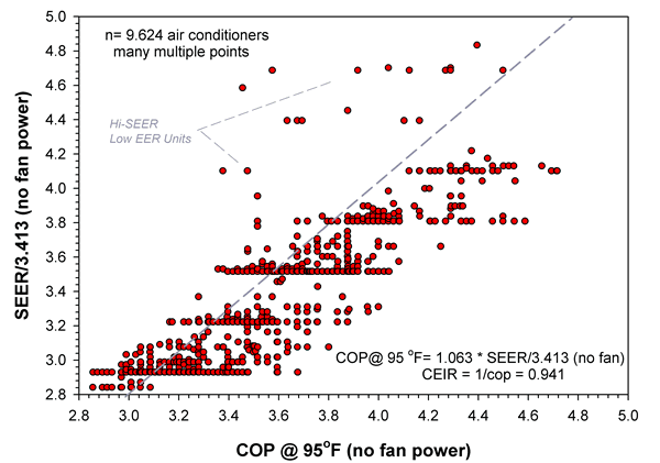
Figure 1. Plot of COP95 vs. SEER/3.413 for air conditioners and heat pumps with default fan power removed.
The data set used for the analysis shown in Figure 1 is constructed such that air handler fan power is not included in the input energy use, yielding a performance parameter, the reciprocal of which can be directly used as input to DOE-2, which requires a value named Energy Input Ratio (EIR – the reciprocal of COP, excluding air handler fan power). Within the ARI test procedure, when the unit includes an indoor blower system, the actual indoor fan power must be used in the calculation. The default value can only be used when an indoor blower is not included with the equipment. Nevertheless, the ARI test does not specifically isolate measured fan power, which is a required quantity to simulate air conditioner and heat pump systems in DOE-2. As such, the ARI default value of 0.365 watts per cfm of air handler airflow is used to determine EIR for DOE-2 input. Use of the ARI value will likely yield higher than actual SEER values, except in the case of the most efficient motors, because the ARI default blower power is significantly lower than that used by typical units (Proctor & Parker, 2000). It would be preferable if the ARI procedures required that fan power be specified and accounted on a unit-by-unit basis but this is not the case. Thus, the ARI air handler blower value of 0.365 W/cfm was subtracted from the input energy for each system.
Heating Seasonal Performance Factor (HSPF)
The Heating Seasonal Performance Factor or HSPF, is determined in an analogous fashion to SEER, but in heating mode. As defined, it is the total heat pump useful heating output during its normal seasonal use divided by the total electrical power input. Here test data is obtained at three differing outdoor test conditions: 47ºF, 35ºF and 17ºF. Performance is interpolated at these points with the results applied against appropriate weather bin data to obtain seasonal performance. The labeled HSPF on heat pumps is that for Climate Zone IV,. Similar to cooling, a part load degradation coefficient is used to evaluate the impact of system cycling under less than design load conditions. Also similar to cooling operation, manufacturers use fan time delay and refrigerant migration prevention to reduce part load losses in modern equipment. However, CD values tend to be somewhat higher for heating although there is less empirical data (Baxter and Moyers, 1985). CD values of 0.15-0.20 may be more common. A detailed assessment by Miller (1985) found that a 90% runtime fraction with a typical heat pump at 50ºF outdoors resulted in an 11% drop in capacity and 7% lower COP than steady state operation. At a 20% runtime fraction heat output was degraded by 35% with COP reduced by 30%
Within the test protocol, the performance of the system can require additional auxiliary strip heat in colder climates. However, the way in which capacity of the system is determined relative to the actual design load, which is arbitrarily reduced by 23% to account for solar and internal gains, serves to reduce the frequency with which strip heat will be encountered -- particularly for systems operated at a more common 68ºF setpoint than the 65ºF setpoint intrinsically assumed within the ARI procedure. This assumption remains a significant upward bias within the overall procedure since most homes will operate at higher heating interior temperatures than 65ºF.
When operating in heating mode, heat pumps require periodic defrosting of ice build-up on the outdoor unit coils. A test is performed to evaluate the system performance impact of the defrost cycle (frost accumulation test). Although some units now use demand defrost schemes, the majority of air source heat pumps use a compressor timer, which activates up to a 10 minute defrost cycle when the compressor has operated for 50-90 minutes.
There are also several other aspects that artificially benefit the HSPF rated performance compared with that which will be encountered in the field. These are summarized briefly below:
- Whereas the defrost operation is typically based on the compressor runtime in real systems, the ARI procedure assumes there is no defrost operation below 17ºF where defrost operation will, in fact, be most often triggered due to extended compressor operation (see Section 4.2.1.3, ARI 210/240).
- Although the vast majority of air-source heat pumps operate auxiliary strip heat during the defrost cycle to prevent "cold blow," the ARI procedure specifically requires that strip resistance heaters be prevented from operating during the frost accumulation test. (Section 4.2.1.3). This is important since such operation of strip heat during the 3-10 minute defrost cycles satisfies part of the house heating load at a lower efficiency that is not reflected in the ARI procedure.
- To achieve better performance in the most severe climate, the ARI procedure computes a smaller building load for the colder Climate Zone V than it does in the more moderate climate zones (I - IV and VI; see equation for BL (Ti) in Section A5.2.1). This results in much lower use of strip heat than would otherwise be encountered in the coldest locations. Conversely, the ARI procedure intrinsically assumes that homes in the mildest locations (Zone I) are just as well insulated as those in Zone IV.
- Finally, beyond standard test conditions, while lower than nominal indoor unit coil air flow will actually increase latent heat removal in cooling mode, there is no such compensation in heating mode. All reductions to system heating capacity due to low coil airflow are a loss to system operating efficiency, generally resulting in increased strip resistance backup.
Figure 2 shows data for nameplate HSPF with comparisons of the compressor COP at 47ºF against the nameplate HSPF/3.413 with fan power removed. Data is shown for 5,549 units with the trend line superimposed on the data.
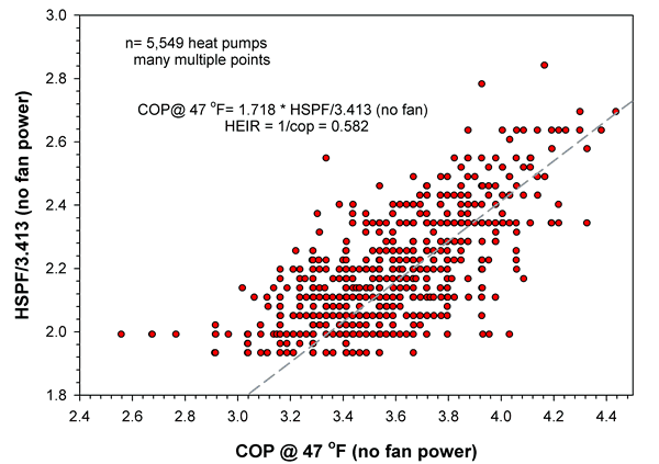
Figure 2. Plot of COP @ 47ºF against HSPF/3.413 with fan power removed from Year 2000 heat pumps.
Evaluation of Climate Related Impacts on Heating and Cooling Performance
To study the climate impacts on standard heat pumps, this study uses EnergyGauge® USA 2.21 (containing a modified DOE-2.1E hourly building simulation engine ) and the Henderson, et.al. (2000) heat pump model to predict the performance of air source heat pumps across the U.S. The program implicitly accounts for internal and solar gains on an hourly basis. The many assumptions associated with the heat pump operation (e.g., defrost method, limit temperatures and crankcase heat) were set to approximate standard current equipment and were employed within a prototype building as detailed below. The heating and cooling system size was varied for each particular building and climate as determined by building loads calculated by Manual J, 7th Edition sizing procedures (ACCA, 1986).
Climate Data and Prototypical Buildings
To address the variations of climate in the U.S., a total of 15 climate locations were simulated. The locations chosen were based on a cluster analysis of North American climates. This procedure considered heating and cooling degree days, solar radiation (T, the dimensionless ratio of annual extraterrestrial solar radiation to that received at the surface on a horizontal plane) and latent enthalpy hours (LEH, an indicator of humidity) for all typical meteorological year data for 125 standard metropolitan statistical areas in the U.S. (Anderson et al., 1984). The 15 chosen locations are Detroit, New York, Los Angeles, Las Vegas, Atlanta, Houston, Ft. Worth, San Francisco, St. Louis, Minneapolis, Miami, Seattle, Fresno, Denver and Phoenix. The sites cover the gamut of meteorological variation within the United States including hot/cold, sunny/cloudy and humid/arid climate types. Descriptions of the climates along with the ARI classifications are summarized in Table 1.
Table
1
Climatological Description of Locations Used for Analysis
Site Location |
Heating
Degree Days |
Cooling
Degree Days |
99%
Design T |
1%
Design T |
ARI
Climate Zone |
| Miami, FL | 149 |
4361 |
50º |
90º |
I |
| Houston, TX | 1525 |
2893 |
31º |
93º |
I |
| Ft. Worth, TX | 2370 |
2568 |
24º |
98º |
II |
| Phoenix, AZ | 1125 |
4189 |
27º |
108º |
II |
| Los Angeles, CA | 1274 |
679 |
45º |
81º |
III |
| Atlanta, GA | 2827 |
1810 |
23º |
91º |
III |
| Las Vegas, NV | 2239 |
3214 |
30º |
106º |
III |
| St. Louis, MO | 4758 |
1561 |
8º |
93º |
III |
| New York, NY | 4947 |
949 |
17º |
89º |
IV |
| Seattle, WA | 4797 |
173 |
28º |
81º |
IV |
| Fresno, CA | 2447 |
1963 |
32º |
101º |
IV |
| Detroit, MI | 6442 |
736 |
5º |
87º |
V |
| Minneapolis, MN | 7876 |
699 |
-11º |
88º |
V |
| Denver, CO | 6128 |
696 |
3º |
90º |
V |
| San Francisco, CA | 2862 |
142 |
39º |
78º |
VI |
Sources: ASHRAE 2001 Handbook of Fundamentals, Chapter 27. National Climatic Data Center, 1971-2000 Normals, The National Oceanic and Atmospheric Administration’s (NOAA), Asheville, NC. ARI/Standard 210/240-2003, Air Conditioning & Refrigeration Institute, Arlington, VA Section A6.2.5.
A Prototype building was created for the 15 climatic locations with simulations run using TMY2 meteorological data (Marion and Urban, 1995). To capture regional variation, the prototype had its required insulation levels varied by climate location according to the Chapter 4, IECC 2000 code minimums (IECC, 1999). A crawlspace type building was assumed since this type exists across climates in the United States. The procedures recommended by Winkelman (2000) were used to calculate foundation/ground heat transfer.
A single-story octagonal floor plan of 2,000 square feet was used for the analysis. The frame-on-crawlspace, octagonal plan was chosen to provide for a solar-neutral configuration such that all windows, walls, doors and roofs are distributed equally in all eight orientations. Building geometry was held constant across climates so that simulated differences could be attributed solely to climate and equipment nameplate efficiency.
All envelope insulation values and window characteristics were determined in accordance with the provisions of Chapter 4, IECC 2000 so as to represent the minimum code requirements (IECC, 1999).
Three occupants were assumed with typical electrical appliances and associated energy use. The specific end-use electrical demand profiles were taken from sub-metered appliance load data gathered from a large sample of homes in the Pacific Northwest (Pratt et al., 1989), but with only 90% of the loads assumed to take place within the conditioned space. The methodology is more fully described in Huang (1987).
The specific heat pump related assumptions used with the DOE-2 simulation are given in Table 2. The heating EIR (Energy Input Ratio or 1/COP47) and Cooling EIR values come from an evaluation of the data for several thousand air conditioners and heat pumps listed in the California Energy Commission appliance database. As is most popular with manufacturers, the heat pump has timed reverse-cycle defrost beginning when the outdoor temperature drops below 40oF. The heat pump provides heating down to 0oF prior to exclusive use of the back-up strip heat elements. Auxiliary strip heat is used when the outdoor temperature is lower than 50oF if the thermostat is not satisfied. Part load ratio curves developed by Henderson, et.al (2000) were utilized within the software model.
The efficiency of the indoor blower is assumed to be 0.5 W/cfm for standard fans with standard PSC motors based on numerous field data on actual performance (Proctor and Parker, 1998). For higher efficiency systems with SEER => 13.5 and HSPF => 8.5, the indoor blower was assumed to be an electronically commutated motor (ECM) with an efficiency of 0.375 W/cfm.
Table
2
Default Values for DOE-2 HVAC Test Runs as Specified within DOE-2.1E
| DOE-2 Keyword: | Description (units) | Value |
| HEATING-EIR | Heat Pump Energy Input Ratio compressor only (1/cop) | 0.582*(1/(HSPF/3.413)) |
| COOLING-EIR | Air Conditioner Energy Input Ratio compressor only (1/cop) | 0.941*(1/(SEER/3.413)) |
| DEFROST-TYPE | Defrost method for outdoor unit (Reverse cycle) | REVERSE-CYCLE |
| DEFROST-CTRL | Defrost control method (Timed) | TIMED |
| DEFROST-T | Temperature below which defrost controls are activated (ºF) | 40º |
| CRANKCASE-HEAT | Refrigerant crankcase heater power (kW) | 0.05 |
| CRANK-MAX-T | Temperature above which crankcase heat is deactivated (ºF) | 50º |
| MIN-HP-T | Minimum temperature at which compressor operates (ºF) | 0º |
| MAX-HP-SUPP-T | Temperature above which auxiliary strip heat is not available (ºF) | 50º |
| MAX-SUPPLY-T | Maximum heat pump leaving air temperature from heating coil (ºF) | 105º |
| MIN-SUPPLY-T | Minimum cooling leaving air temperature from cooling coil (ºF) | 55º |
| SUPPLY-KW | Indoor unit standard blower fan power (kW/cfm) | 0.0005 |
| SUPPLY-DELTA-T | Air temperature rise due to fan heat, standard fan (ºF) | 1.580 |
| SUPPLY-KW | Indoor unit standard blower fan power, high efficiency fan (kW/cfm) | 0.000375 |
| SUPPLY-DELTA-T | Air temperature rise associated due to fan heat, high efficiency fan (ºF) | 1.185 |
| COIL-BF | Coil bypass factor (dimensionless) | 0.241 |
| Other parameters: | ||
| Part load performance curves | Compressor part load performance curves | Henderson,
et.al. |
| Heating system size | Installed heat pump size (Btu/hr) | Determined
by Manual J |
| Coil airflow | Indoor unit air flow (cfm) | 360
cfm/ton |
| Cooling system size | Installed air conditioner size (Btu/hr) | Determined
by Manual J |
Although the authors are aware of the common practice of over sizing heating and cooling equipment (e.g., James et al, 1977), this was not done within this study. Instead, we used the results of a Manual J (7th Edition) calculation to size the heating and cooling equipment (ACCA, 1986).
Results
Not surprisingly, the analysis showed that the derived operating efficiency from the simulation results declined with winter climate severity. A statistical analysis was conducted to regress the operating performance data against the 99% winter design temperature (2001 ASHRAE Handbook) and the manufacturer’s HSPF performance rating. Similarly, the seasonal cooling system performance was well represented by the 1% summer design temperature and the manufacturer’s SEER rating. Two sets of regression analysis were performed for each of the seasonal performance ratings – the first set for the lower-efficiency range (SEER < 13.5 and HSPF < 8.5) and the second for higher-efficiency range. This is necessitated by the modeling assumptions made for blower performance, where higher efficiency units were assumed to have high-efficiency ECM or equivalent blower motors. This effect had a greater impact in cooling mode (where the reduction in fan heat effectively reduces the cooling load).
Using only the ASHRAE 1% or 99% design temperatures (Temp) and the nameplate HSPF or SEER rating, all four regressions were able to achieve regression coefficients (R-square) greater than 0.96. Figures 3 shows the results of the regression analysis for heating season performance (HFPF) for the higher efficiency HSPF range. The regression plot results for the lower efficiency HSPF and SEER ranges are virtually identical to those of the higher efficiency ranges and are not shown here for space considerations.
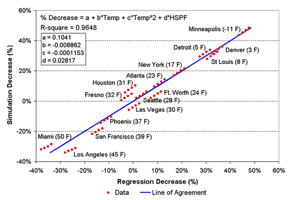
Figure 3. Change in nameplate HSPF as a function of winter design temperature showing agreement between the simulated decrease and that predicted by the regression equation for HSPF => 8.5.
The analysis shows that the 1% design temperature and nameplate HSPF are sufficient to achieve good correlation (R-square in excess of 0.96 for all cases). It is also clear that a significant decrease in nameplate HSPF (~50%) will occur in sever climates like Minneapolis, MN. However, the results also show that in very mild climates like Miami, FL, the achieved performance will exceed the nameplate performance. Note also that four data points characterize each climate data group, with larger HSPFs producing greater decreases in HSPF as compared with the nameplate data.
The general regression equation and coefficients for HSPF are as follows:
%Decrease = a + b*Temp + c*Temp2 + d*HSPF
Coeff: |
HSPF
< 8.5 |
HSPF
=> 8.5 |
a
= |
0.1392 |
0.1041 |
b
= |
-0.008460 |
-0.008862 |
c
= |
-0.0001074 |
-0.0001153 |
d
= |
0.02280 |
0.02817 |
R-Square
= |
0.9649 |
0.9648 |
Figure 4 shows the similar results for cooling season performance for the higher efficiency SEER range.
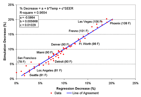
Figure 4. Change in nameplate SEER as a function of summer design temperature showing agreement between the simulated decrease and that predicted by the regression equation for SEER => 13.5.
The SEER data do not show the same degree of decrease compared to nameplate SEER as do the HSPF data. The simple explanation is that the air conditioning cycle does not have an analog to the strip resistance backup of the heating cycle. It is also interesting to note in the above data that there are no climates where air conditioners perform better than their nameplate value. Again, climate clearly has a major impact on realized performance, with Las Vegas, NV and Phoenix, AZ showing relative large performance decreases (~22% compared with the nameplate rating).
The general regression equation and coefficients for SEER are as follows:
%Decrease = a + b*Temp + c*SEER
Coeff: |
SEER
< 13.5 |
SEER
=> 13.5 |
a
= |
-0.5655 |
-0.5864 |
b
= |
0.005414 |
0.005668 |
c
= |
0.01039 |
0.01029 |
R-Square
= |
0.9624 |
0.9654 |
The SEER calculations assume an 80oF indoor temperature against the 78oF indoor temperature and hourly location specific outdoor temperatures simulated in our analysis. In particular, the greater assumed fan power adversely affects “operating efficiency” relative to nameplate SEER ratings. The severity of outdoor temperatures also impact cooling efficiency particularly in the hottest locations (e.g., Phoenix).
Where only nameplate SEER and HSPF and climate data are available (the usual case for most energy evaluations that compare alternatives), the results of the above analysis are useful for understanding and accounting for the impacts of climate on heat pump performance. Where energy use estimates are needed, a climate specific performance factor (nameplate rating * [1-%Decrease]) will provide a more accurate energy estimate than will the nameplate rating.
Figure 5 summarizes the fundamental results across climates for heating and cooling superimposed on the map of ARI climate zones around the contiguous United States. In general, the simulations predict lower than rated performance for both HSPF and SEER – likely in large part due to the less advantageous indoor temperature and fan power assumptions. The calculations for HSPF intrinsically assume a 65oF interior air temperature as opposed to 68oF used in the simulations. Even so, in the milder climates of Miami, Los Angeles, San Francisco and Phoenix the “operating efficiency” was actually greater than the nameplate HSPF rating.
Conclusions
A simulation analysis was conducted on variation in seasonal heating and cooling performance of air-source heat pumps as a function of local climate conditions. Although the conventional Seasonal Energy Efficiency Ratios (SEER for cooling) and Heating Seasonal Performance Factor (HSPF) values for systems sold in the U.S. have a single published value based on performance in ARI Region IV one would expect performance to vary with climate severity – particularly for heating where winter conditions vary widely across the United States.
As expected, the analysis shows that the seasonal heating and cooling performance of heat pumps and air conditioners change substantially with climate. Simulation data indicate that statistical association with the site-specific summer and winter design temperatures can capture much of this variation in seasonal performance. Equations relating these factors are presented. Over the range of climates, actual SEER was found to vary by as much as 22% from nameplate values with the hottest locations showing most decrease in performance. However, the variation in HSPF was much greater. The climate related HSPF was found to be as much as 40% better or 50% worse than the published values depending on site winter climate.
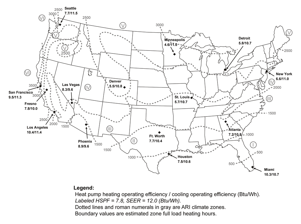
Figure 5. Map of ARI climate zones showing results of simulations in representative climates. (click for larger image)
References
ACCA, Air Conditioning Contractors of America: Manual J _ Load Calculation for Residential Winter and Summer Air Conditioning, Seventh Addition, 1986.
ARI, 2003. Standard 210/240: Unitary Air Conditioning and Air Source Heat Pump Equipment, Air Conditioning and Refrigeration Institute, Arlington, VA.
ASHRAE, 2001. Handbook of Fundamental, American Society of Heating, Refrigerating, and Air-Conditioning Engineers, Inc., Atlanta, GA.
EIA, 2001. Housing Characteristics 2001, DOE/EIA-0314, Energy Information Administration, Washington D.C.
EPRI, 1980. Final Report: ERPRI Project RP-1351, Electric Power Research Institute, Palo Alto, CA.
IECC, 1999. International Energy Conservation Code 2000, International Code Council, Inc., Falls Church, VA.
Anderson, B., W.I. Carroll, and M.R. Martin, 1986. “Aggregation of U.S. population centers using climate parameters related to building energy use,” Journal of Applied Meteorology, Vol. No. 25, 1986.
Andrews, L., W. Gavelis, M. King, J. Jennings, Super Good Cents Performance Analysis: Progress Report, prepared Bonneville Power Administration, Synergic Resources Corporation/ Columbia Information Systems. CIS/SRC Report No. 7343-R3, April 1989
Baxter, V.D. 1981. ACES: Final Performance Report December 1, 1978 through September 15, 1980, ORNL/CON-64, Oak Ridge, TN, Oak Ridge National Laboratory.
Baxter, V.D. and Moyers, J.C., 1985. “Field-Measured Cycling, Frosting, and Defrosting Losses for High-Efficiency Air-Source Heat Pump,” ASHRAE Transaction, Vol. 91, Part 2B, pgs. 537-554.
Bouchelle, M.P., D S Parker, M T Anello, and K M Richardson, 2000. "Factors Influencing Space Heat and Heat Pump Efficiency from a Large-Scale Residential Monitoring Study." Proceedings of 2000 Summer Study on Energy Efficiency in Buildings, American Council for an Energy-Efficient Economy, 1001 Connecticut Avenue, Washington, DC, Vol. 1, p. 225.
Bullock, C. 1978. "Energy Savings Through Thermostat Setback with Residential Heat Pumps," ASHRAE Transactions, Vol. 84, 2: 352-363, Atlanta, GA: American Society of Heating, Refrigeration and Air Conditioning Engineers.
Dougherty, Brian P., “New Defaults for the Cyclic Degradation Coefficient Used in Rating Air Conditioners and Heat Pumps,” NIST, ASHRAE Seminar 40, July 2003.
Eckman, T., 2000. “Super Good Cents Metered Data Report: Spreadsheet,” Northwest Power Planning Council, Portland, OR, August 2000.
Groff, G.C., C.E. Bullock and W.R. Reedy, 1978. “Heat Pump Performance Improvements for Northern Climate Applications,” 13th Proceedings of the Intersociety Engineering Conversion Conference, San Diego, CA, Aug 20-25, 1978.
Harris, W.S., et al., 1965. "Estimating Energy Requirements for Residential Heating," ASHRAE Journal, Vol. 7, No. 10, October 1965.
Henderson, H.I., D.S. Parker and Y.J. Huang, 2000. “Improving DOE-2's RESYS Routine: User Defined Functions to Provide More Accurate Part Load Energy Use and Humidity Predictions,” Proceedings of 2000 Summer Study on Energy Efficiency in Buildings, Vol. 1, p. 113, American Council for an Energy-Efficient Economy, 1001 Connecticut Avenue, Washington, DC.
Huang, J., 1987. Methodology and Assumptions for Evaluating Heating and Cooling Energy Requirements in New Residential Single Family Buildings, LBL-19128, Berkeley, CA, Lawrence Berkeley National Laboratory.
James, P., J.E. Cummings, J. Sonne, R. Vieira, J. Klongerbo, “The Effect of Residential Equipment Capacity on Energy Use, Demand, and Run-Time,” ASHRAE Transactions 1997, Vol. 103, Pt. 2, American Society of Heating, Refrigerating, and Air-Conditioning Engineers, Inc., Atlanta, GA.
Kavanagh, S.P., 2002. “Limitations of SEER for Measuring Efficiency,” ASHRAE Journal, July 2002.
Marion, W. and K. Urban, 1995. User’s Manual for TMY2: Typical meteorological years. Golden, CO, National Renewable Energy Laboratory.
Miller, W.A., 1985. “The Laboratory Evaluation of the Heating Mode Part-Load Operation of an Air-to-Air Heat Pump,” ASHRAE Transactions, Vol. 91, Part 2B, pgs. 524-536.
Miller, R.S. and H. Jaster, 1985. Performance of Air Source Heat Pumps, prepared by the General Electric Company for the Electric Power Research Institute, EM-4226, Palo Alto, CA.
Nicolich, M.J., 1977. “Residential Heat Pump Use: Saving Electrical Energy,” ASHRAE Journal, Vol. 19, No. 12.
O’Neal, D., 2002. “Personal communication,” Department of Mechanical Engineering, Texas A&M University, 16 December, 2002.
Orth, Jr., L.M. and D.C. Hamilton, 1976. Thermodynamic and Economic Analysis of Improved Residential Climate Control Systems, Prepared for Louisiana Power and Light Co., Dept. of Mechanical Engineering, Tulane University, Aug. 1976.
Parken, W.H., R.W. Beausoliel and G.E. Kelly, 1977. “Factors Affecting the Performance of a Residential Air to Air Heat Pump,” ASHRAE Transactions, Vol. 83, Pt. 1.
Parker, D. S., 2002. "Research Highlights from a Large Scale Residential Monitoring Study in a Hot Climate." Proceedings of International Symposium on Highly Efficient Use of Energy and Reduction of its Environmental Impact, pp. 108-116, Japan Society for the Promotion of Science Research for the Future Program, JPS-RFTF97P01002, Osaka, Japan, January 2002.
Pratt, R.G., C.C. Connor, E.E. Richman, K.G. Ritland, W.F. Sandusky, and M.E. Taylor, 1989. Description of electric energy use in single-family residences in the Pacific Northwest: End use load and consumer assessment (ELCAP), DOE/BP-13795-21, Pacific Northwest Laboratory, Richmond, WA.
Proctor, J and D Parker, 2000, Hidden Power Drains: Trends in Residential Heating and Cooling Fan Watt Power Demand.” Proceedings of 2000 Summer Study on Energy Efficiency in Buildings, American Council for an Energy-Efficient Economy, 1001 Connecticut Avenue, Washington, DC.
Reedy, C.S. and S.A. Daniels, “Analysis of Heat Pump Performance in the Northeastern U.S.A.,” Proceedings of the 27th Intersociety Energy Conversion Engineering Conference, Vol. 3, Society of Automotive Engineers,IECEC-92, San Diego, CA, 1992.
Rettberg, R.J., 1980. “Cooling and Heat Pump Heating Season Performance Effects Evaluation Models,” ASHRAE Transactions, Vol. 86, Pt. 1.
Wildin, M.W., A. Fong, C. Wilson and J. Nakos, 1978. “Analysis of the Effects of Cycling on Energy Use of Cycling on Energy Use of Installed Air-to-Air Heat Pumps in Albuquerque, New Mexico,” Department of Mechanical Engineering, University of New Mexico, in Conference on Heat Pump Technology, Stillwater, OK, 10 April 1978.
Winkelmann, F., 1998. "Underground Surfaces: How to Get Better Underground Surface Heat Transfer Calculation in DOE-2.1E," DOE_2 USER News, Vol. 19, No. 1, p. 6-13, Lawrence Berkeley National Laboratory, Berkeley, CA.
© 2007-2014 University of Central Florida. The Florida Solar Energy Center (FSEC)
is a research institute of the
University of Central Florida.
For more information about FSEC, please contact us or learn more about us.
Find us on Facebook!