

Reference Publication: Henderson, H., Parker, D., Huang, Y., "Improving DOE-2's RESYS routine: User Defined Functions to Provide More Accurate Part Load Energy Use and Humidity Predictions", Proceedings of 2000 Summer Study on Energy Efficiency in Buildings, American Council for an Energy-Efficient Economy, 1001 Connecticut Avenue, Washington, DC., August 2000. Disclaimer: The views and opinions expressed in this article are solely those of the authors and are not intended to represent the views and opinions of the Florida Solar Energy Center. |
Improving
DOE-2’s RESYS routine:
User Defined Functions to Provide More Accurate
Part Load Energy Use and Humidity Predictions
Hugh
I. Henderson, Danny Parker, Yu J. Huang
CDH Energy
Corp., Florida Solar Energy Center (FSEC), Lawrence Berkeley Laboratory
FSEC-PF-409-00
ABSTRACT
In hourly energy simulations, it is important to properly predict the performance of air conditioning systems over a range of full and part load operating conditions. An important component of these calculations is to properly consider the performance of the cycling air conditioner and how it interacts with the building. This paper presents improved approaches to properly account for the part load performance of residential and light commercial air conditioning systems in DOE-2. First, more accurate correlations are given to predict the degradation of system efficiency at part load conditions. In addition, a user-defined function for RESYS is developed that provides improved predictions of air conditioner sensible and latent capacity at part load conditions. The user function also provides more accurate predictions of space humidity by adding “lumped” moisture capacitance into the calculations. The improved cooling coil model and the addition of moisture capacitance predicts humidity swings that are more representative of the performance observed in real buildings.
Introduction
In hourly energy simulations, it is important to properly predict the performance of air conditioning systems over a range of full and part load operating conditions. An important component of these calculations is to properly consider the performance of the air conditioner and how it interacts with the building.
Energy simulation programs such as DOE-2 use well understood calculation procedures based on "first principles" to determine the heat transfer through the building envelope, or loads. However, the performance of the HVAC equipment is typically determined using empirical functions that predict system energy use and capacity as a function of operating conditions such as outdoor and indoor temperature, humidity, and equipment loading. DOE-2 includes empirical functions in the form of multi-variable polynomials for numerous types of HVAC systems (Buhl et al 1993). These curves typically "extend" the nominal, or design performance of the system to off design conditions. DOE-2 provides default empirical models for these systems that have been developed over the last 20 years. Many of these curves are based on equipment that may no longer reflect products that are available in the market. In other cases the default curves may have been developed based on data over a narrow range of conditions that are no longer appropriate.
Perhaps the most complicated models are required for the simplest system: the residential or small commercial air conditioner. This direct-expansion cooling unit cycles on and off to meet the load based on the space temperature sensed by a thermostat. The relatively complex dynamics of the DX air conditioner and the thermostat are modeled in hourly simulation programs by using simplified empirical functions that predict the degradation in efficiency (or added energy use) for hours when the unit operates for only part of the time.
Another complicating factor is that the DX air conditioner provides both sensible cooling and moisture removal (i.e., latent capacity). The mix of latent and sensible capacity provided by the unit depends on several factors including ambient temperature, the air flow rate, and the psychrometric conditions entering the evaporator coil
-
More realistic predictions of part load efficiency degradation and its impact on air conditioner energy use.
-
Better predictions of air conditioner latent and sensible capacity over a range of operating conditions.
-
The addition of moisture capacitance into DOE-2's zone moisture balance calculations to improve the prediction of time-varying space humidity levels.
The following section addresses the issue of part load efficiency degradation for DX air conditioners and suggests improved FEIR-PLR functions for use in DOE-2. Then a more rational DX air conditioner model is described and the method for integrating the model into the DOE-2 RESYS routine as a user defined function is presented.
Part Load Efficiency Degradation for Cycling Equipment
It is generally convenient to express part load effects in terms of degradation of efficiency under part load. Parken et al (1977) at NIST (formerly the National Bureau of Standards) referred to the normalized efficiency degradation as the part load factor, or PLF.
![]() (1)
(1)
This nomenclature is also used in the SEER test procedures (DOE 1979). PLF of a cycling HVAC system depends on:
- the response of the cooling system at startup (usually defined by a time constant or dead time),
- the cycling rate of the equipment (usually defined by thermostat characteristics and to a lesser extent the building thermal mass).
Parken and his co-workers at NIST were the first to recognize that these two factors could be combined to form a part load correlation. They used this concept to develop the part load degradation coefficient (C d) used today in the SEER rating procedure (equation 2). They verified the concept with both laboratory and field data (Parken et al 1985). PLR, the part load ratio, is defined as the ratio of the hourly load and available capacity.
![]() (2)
(2)
Henderson and Rengarajan (1996) showed that the theoretical part load efficiency curve could be summarized in the form of Equation 3. Successive substitution is required to solve for PLF as a function of PLR and the parameters N max and t.
![]() (3a)
(3a)
where : |
||
and: |
N max = Maximum cycling rate of the cooling system / thermostat (cycles/h) | |
| t = Time constant of air conditioner cooling capacity (hrs) | ||
Figure 1 shows that the theoretical function (eqn. 3) closely matches the linear C d model (eqn. 2). The default value of C d in the SEER rating procedure is 0.25. This value corresponds to time constant ( t or tau) of 76 seconds for the air conditioner capacity at startup, and a maximum thermostat cycling rate (N max) of 3.125 cycles per hour. For systems with less degradation (i.e., smaller C d or t) the linear curve is even more closely matched to the theoretical model.
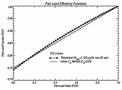
Figure 1 .
Comparing Theoretical and Linear Part Load Models
Modern air conditioner and heat pump systems typically have time constant of 40 to 60 seconds. As a result, values of C d measured for typical systems tested according Tests C and D of the SEER procedure are in the range of 0.1 to 0.2. Thermostat cycling rates are also generally lower than the default value of 3.125 assumed in the rating procedure. An average cycling rate of 30 Florida homes was found to be 2.5 cycles per hour (Henderson et al 1991). This further reduces the effective value of C d.
For systems that use power when the system is off, it is sometimes desirable to include the impact of this power into the part load degradation curve. Off cycle power can include crankcase heaters, controls, or other parasitic uses.
Bonne et al (1980) and Miller and Jaster (1985) both showed that, when off-cycle power consumption is considered, the part load efficiency curve is modified as given by equation (4) and PLF' is the resulting factor considering off-cycle power (where PLF is from equation 2 or 3). The off-cycle power use is expressed as a fraction of on-cycle power use (pr).
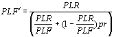 (4)
(4)
Figure 2 shows that considering even small amounts of off-cycle power has a dramatic impact on efficiency at low load conditions. A value of 0.01 for pr corresponds to about 40 Watts of off-cycle power for a typical 3 ton AC system, while 0.03 corresponds to 120 Watts.
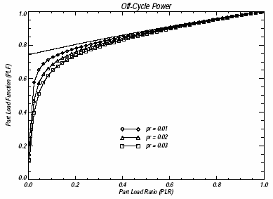
Figure 2 .
The Impact of Off-cycle Power on PLF
DOE-2's Approach to Part Load Degradation
DOE-2 includes several correlation curves that predict the energy use of systems under part load conditions. Because DOE-2 was first developed for larger buildings that typically use chillers, the efficiency degradation is expressed it terms of the Energy Input Ratio (EIR). EIR is the inverse of efficiency, or COP, and is the dimensionless equivalent of kW per ton. The part load correlations for DOE-2 are polynomials that predict EIR as function of PLR. Then the EIR-FPLR factor is multiplied by the nominal power of the machine to find its part load energy use. The EIR-FPLR functions can be rearranged to find PLF with equation 5.
![]() (5)
(5)
Figure 3 shows the DOE-2 default curves for part load performance of various types of equipment plotted in the PLF form. Table 1 lists the DOE-2 SYSTEMS and PLANT equipment that use these curves. Due to the inverted form of the equation, all five curves show the following behavior:
-
the part load efficiency goes to zero as PLR approaches zero,
-
the slope of the curves is strongly a function of loading (i.e., PLR)
The curve for residential cooling shows the most part load degradation, followed by the boiler and heat pump heating curves. The furnace and PSZ cooling curves show the least amount of part load degradation. Even though these curves are a simple linear model of EIR as function of PLR, when inverted using equation 5 the functions predict a significant amount of degradation that was not readily apparent in the original EIR form.
Table 1 . Default Part Load Curves in DOE-2
| Description | Curve Name | Curve No | DOE-2 Systems |
| Residential Cooling | COOL-EIR-FPLR | 16,17,20 | RESYS,PTAC,HP |
| Commercial Cooling | COOL-EIR-FPLR | 18, 128 | PSZ,PMZS,PVAVS PVVT |
| HP Heating | HEAT-EIR-FPLR | 61,62,65, 75,116 | RESYS, PSZ, PTAC, PVAVS, HP, WTR-CC, PVVT |
| Furnace | FURNACE-HIR-FPLR | 111 | any fuel-fired furnace |
| Boiler | BOILER-HIR-FPLR | BLRHIR2 | HP (WLHP system) HW and Steam Boiler Plants |
Figure 3 .
Default Curves for DOE-2 Presented in the PLF vs. PLR Form
Recommended Curves for Residential and Light Commercial Cooling Systems
Figure 4 shows the range of part load performance that might be expected for a residential cooling system. Table 2 lists the corresponding EIR coefficients. The two plots show curves that include the impact with and without off-cycle power. The default RESYS curve (without off-cycle power adjustments) is also shown on each plot for reference.
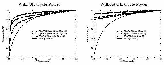
Figure
4 . Recommended Parameters for a Typical
AC System
Compared to Default DOE-2 Curve (without off-cycle power)
Table 2 . EIR Coefficients For “Typical AC” in Figure 4
| Coefficients for EIR-FPLR = a + b × PLR + c × PLR 2 + d × PLR 3 | ||||
a |
b |
c |
d |
|
| Curves with Off-Cycle Power | ||||
| “Typical AC” ( N max=2.5, tau=60, pr=0.01) | 0.0101858 |
1.18131 |
-0.246748 |
0.0555745 |
| “Good AC” ( N max=2.5, tau=60, pr=0.01) | 0.00988125 |
1.08033 |
-0.105267 |
0.0151403 |
| “Poor AC” ( N max=3, tau=60, pr=0.03) | 0.0300924 |
1.20211 |
-0.311465 |
0.0798283 |
| Curves without Off-Cycle Power | ||||
| “Typical AC” ( N max=2.5, tau=60) | 0.000352822 |
1.19199 |
-0.246716 |
0.0546566 |
| “Good AC” ( N max=2.5, tau=60) | 4.28122e-005 |
1.09001 |
-0.103863 |
0.0138504 |
| “Poor AC” ( N max=3, tau=60) | 0.000582243 |
1.23565 |
-0.313841 |
0.0780726 |
To implement these curves in DOE-2, use the commands:
newPLR CURVE-FIT TYPE=CUBIC COEF=(a,b,c,d) ..
COOL-EIR-FPLR=newPLR ..
The “Typical AC” is assumed to have a time constant of 60 seconds at startup, which is typical of values reported in the literature and summarized by Henderson (1992), with values ranging from 30 to 80 seconds. The “Good AC”, which might be representative of a system with a liquid line solenoid or other means of off-cycle refrigerant control, is assumed to have a shorter time constant of 30 seconds.
The maximum thermostat cycling rate is assumed to be 2.5 cycles per hour for the “Typical AC” and “Good AC” . This value was the average measured at 30 Florida homes by Henderson et al (1991). By comparison Miller and Jaster (1985) measured values of 1.5 to 3 cycles per hour and recommended 3 as the “worst case”. Parken et al (1985) measured values of 1.6, 2.0, and 2.3 cycles/hr in the cooling mode at their 3 test homes. The “Poor AC” is assumed to have a cycling rate of 3 cycle per hour.
The off-cycle power use is expected to be 1% (0.01), or about 40 Watts with a 3 ton unit for the “Typical AC”. This is close to the value of 1.5% assumed by Bonne et al (1980). The “Poor AC” is assumed to be 3% (0.03), or 120 Watts for a 3 ton unit.
If the curves with off-cycle power are used with DOE-2, then the crankcase heater keyword CRANKCASE-HEAT in RESYS should be set to zero (the default value is 50 Watts). Otherwise, the part load curves without off-cycle power can be used and the crankcase heater power can be specified independently. This approach has the advantage of allowing the crankcase heater to only operate whenever the compressor is off and ambient conditions fall below a specified set point (CRANKCASE-MAX-T = 70 °F by default).
There is not expected to be much difference between new and existing systems. Most research into part load issues was conducted in the 1970’s and 1980’s, though work at FSEC (Henderson 1990) and other places appears to confirm these earlier findings. While the steady state performance of residential AC and HP systems has improved substantially over the last 10 to 15 years, there is little evidence that part load issues have changed for cycling equipment. The transient response at startup is still expected to be similar, with the exception of systems with liquid line solenoid valves or totally closeable electronic expansion valves, which are expected to respond faster since refrigerant is trapped in the condenser. Thermostat manufacturers also still design for maximum cycling rates of 2 to 3 cycles per hour.
Impact of Part Load Degradation
Table 3 summarizes the impact that the improved part load function has on a typical 1,500 ft 2 house in Miami. The default RESYS curves add 24% to the annual energy use of the air conditioner. In contrast, the “Poor” and “Good” AC curves (without off cycle power considered) predict that part load efficiency losses are only 4 and 11%, respectively. Annual losses of 5-10% have generally been shown in the literature from field studies and detailed, small time step simulations (Henderson 1992).
Table 3 . Impact of Part Load Models on Annual Cooling Energy Use in DOE-2
Part Load
Losses (kWh/yr) |
Annual Losses
(%) |
|
| Default RESYS Curves (SDL-C17) | 936 |
24% |
| "Poor" AC (w/o off-cycle power, Figure 4 ) | 417 |
11% |
| "Good" AC (w/o off-cycle power, Figure 4 ) | 170 |
4% |
Miami House with cooling energy use of 3,831 kWh/yr with part load degradation turned off.
A User Function for Improved Humidity Predictions
DX Coil Model
To accurately predict space humidity levels, the air conditioner model must properly predict the split of sensible and latent capacity over a range of operating conditions. It is generally accepted that the total (sensible and latent) capacity of a DX air conditioner is a function of ambient conditions and the entering wet bulb temperature. However, the sensible and latent portions of the total capacity are a function of the psychrometric state point of the entering air, not just the wet bulb alone.
This aspect of cooling coil performance is best described by the apparatus dew point/bypass factor (ADP/BF) approach. This approach is an analog to the NTU-effectiveness calculations used for sensible-only heat exchanger calculations extended to a cooling and dehumidifying coil. BF, by definition, is one minus the heat exchanger effectiveness for both the latent and sensible calculations. For an air-to-refrigerant heat exchanger (where C min/C max=0) BF is defined as:
![]() (6)
(6)
![]() =
constant /cfm (7)
=
constant /cfm (7)
Then the leaving temperature and humidity conditions from the coil are found with the ADP and BF as shown below in equations 8 and 9 below. The humidity ratio w ADP corresponds to saturation conditions at the apparatus dew point.
![]() (8)
(8)
![]() (9)
(9)
The DOE-2 documentation (Version 2.1C Reference Manual) describes the cooling algorithms for the DX systems, including RESYS. The DX cooling models use the ADP/BF approach, but the algorithms make the error of assuming that the bypass factor (BF) is a function of the psychrometric conditions entering the coil (i.e., the DB and the WB) in addition to the air flow rate. The variation of BF is specified by the polynomial functions COIL-BF-FT and COIL-BF-FCFM (the default curves are SDL-C31 & SDL-C41). The dependence of BF on DB and WB does not have a physical basis, as shown by equations 6 and 7. However, eliminating the dependence of BF on DB and WB, and making it a fixed value, actually makes the latent/sensible characteristics of RESYS worse. It appears that the original developers have fit this “non-physical” form of the COIL-BF-FT equation to actual data. The variation of BF with DB & WB actually mimics the variation you might expect for the ADP (or TSURF) at least near design conditions. However, less than rational performance is observed at off-design conditions.
To provide a more physically-based model for the DOE-2 RESYS routine, the ACDX.DXDOE subroutine from ASHRAE’s Secondary Toolkit (Brandemuehl et al 1993) was adapted for use as a user-defined function in DOE-2. The model is also described by Henderson, Rengarajan, and Shirey (1992).
The DX AC routine is a “physically rational” model that predicts the latent and sensible capacity of a cooling coil at off-design conditions. It uses the total capacity and efficiency correlations from DOE-2 (PSZ curves from version 2.1c) along with the bypass factor/apparatus dewpoint (BF/ADP) relations to model performance. The routine uses the nominal capacity, Sensible Heat Ratio (SHR), Energy Efficiency Ratio (EER), at design conditions ( i.e., 80 °F/67 °F entering air, 95 °F ambient, 450 cfm/ton) to construct a performance map for off-design conditions.
The original FORTRAN routine included several iteration loops. However, the implementation as a user-defined function was simplified so that iterations were not required. For instance, the user function can not predict proper power use at dry coil conditions (however, this condition should rarely occur in a residential AC system). Also, a simple correlation is used to relate nominal SHR to the nominal BF instead of iterating to find an exact solution. A curve fit that relates enthalpy and temperature at saturation conditions between 25 °F and 60 °F was also developed to eliminate the need for iterations to find ADP from the leaving enthalpy. These approximations introduce very little error for an air conditioner treating mostly return air in a residential application. The user function is listed in Appendix A.
Moisture Capacitance
In addition to calculating available sensible and latent capacity for the AC cooling coil, the user-defined function also calculates the resulting impact on zone humidity. DOE-2 does not consider moisture storage effects in the building zone. Instead, it calculates the steady-state moisture balance for each hour and solves for the space humidity that achieves a balance. This calculation approach results in humidity levels that are much different than is observed in real buildings and can result in sudden, unrealistic jumps in predicted space humidity conditions. To improve the physical accuracy of simulations, a moisture capacitance model was added to the user-defined function. This model assumes the building has a “lumped” moisture holding capacity, or capacitance (C a), that is a multiple of the interior air mass. Comparisons to more detailed moisture transport/storage models such as FSEC (Kerestecioglu et al 1989) have shown the simple lumped approach yields results similar to more detailed approaches with a lumped moisture capacitance that is equivalent to 20 times the building air mass. To implement moisture capacitance we first start with the mass balance equation:
![]() (10)
(10)
Discretizing the differential equation to an hour and using “forward differencing,” the equation for a residence becomes:
![]() (11)
(11)
Where w i’ is the humidity level for the next hour. Assuming C a is large, then the humidity changes at a rate less than 1 gr/lb per hour. This makes the errors associated with forward differencing small (i.e., latent capacity and infiltration loads are evaluated with w i from the current hour to find the space humidity for the next hour). The implementation of the algorithm in the user-defined function is shown in Appendix A.
Impact on Performance
This simple moisture balance approach yields space humidity trends that are consistent with more detailed moisture capacitance models (Shirey and Rengarajan 1996). Figure 5 compares the resulting humidity level with this new modeling approach to the humidity levels predicted with RESYS. The large fluctuations with RESYS are eliminated with the new approach and the humidity levels more closely match what might be expected for a house in Miami. The addition of capacitance makes the daily humidity swings much more inline field-measured performance.
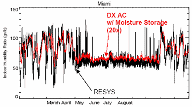
Figure 5 Comparing
Zone Humidity Levels with RESYS
and DX AC/Moisture Storage Approach
Summary
Two approaches to improve the part load performance of cycling air conditioning systems have been developed. Coefficients are given for improved efficiency degradation curves in DOE-2. The new curves reduce the annual efficiency degradation penalty to the 5-10% range compared to unrealistically large 24% penalty that results with the default RESYS curves. A user defined function for RESYS is also developed with improved cooling coil models and moisture capacitance to provide more accurate predictions of space humidity.
References
Bonne, U. Patani, A. Jacobson, R.D. and Mueller, D.A. 1980. Electric-Driven Heat Pump Systems: Simulations and Controls II. ASHRAE Transactions. 86(1) LA-80-5 No. 4. pp 687-705.
Brandemuehl, M., S. Gabel and I. Anderson. 1993. HVAC 2 Toolkit - A Toolkit for Secondary HVAC System Energy Calculations. Prepared for TC 4.7 Energy Calculations. ASHRAE. Atlanta.
Buhl, W.F., B. Birdsall, A.E. Erdem, K.L. Ellington, F.C. Winkelmann, and Hirsch & Associates. 1993. DOE-2 SUPPLEMENT, VERSION 2.1e. LBL34947. November
DOE 1979. Test procedures for central air conditioners including heat pumps. Federal Register Vol. 44, No. 249. pp 76700-76723. December 27, 1979.
Henderson, H.I., 1990. ‘An Experimental Investigation of the Effects of Wet and Dry Coil Conditions on Cyclic Performance in the SEER Procedure,’ Proceedings of USNC/IIR Refrigeration Conference at Purdue University, July, West Lafayette, IN
Henderson, H.I., Rengarajan, K., Raustad, R. 1991. Measuring Thermostat and Air Conditioner Performance in Florida Homes. Research Report #FSEC-RR-24-91. Florida Solar Energy Center, Cape Canaveral, FL. May.
Henderson, H.I., K. Rengarajan, D.B. Shirey, 1992. ‘The Impact of Comfort Control on Air Conditioner Energy Use in Humid Climates,’ ASHRAE Transactions Vol. 98 Part 2, June.
Henderson, H.I. 1992. Simulating Combined Thermostat, Air Conditioner and Building Performance in a House. ASHRAE Transactions. 98(1) January.
Henderson, H. and K. Rengarajan. 1996. A Model to Predict the Latent Capacity of Air Conditioners and Heat Pumps at Part Load Conditions with the Constant Fan Mode. ASHRAE Transactions. 102 (1) January.
Kerestecioglu, A., M. Swami, P. Brahma, L. Gu, P. Fairey, and S. Chandra. 1989. FSEC 1.1 User Manual : Florida Software for Energy and Environmental Calculations, FSEC. August.
Miller , R.S., and Jaster, H. 1985. Performance of Air-Source Heat Pumps, Project 1495-1 Final Report, EPRI EM-4226, Nov.
Parken, W.H., Beausoliel, R.W., and Kelly, G.E. 1977. Factors Affecting the Performance of a Residential Air-to-Air Heat Pump. ASHRAE Transactions. 83(1) No. 4269. pp. 839-849.
Parken, W.H., Didion, D.A., Wojciechowshi, P.H., and Chern, L. 1985. Field Performance of Three Residential Heat Pumps in the Cooling Mode. NBSIR 85-3107, report by National Bureau of Standards, sponsored by U.S. Department of Energy for U.S. Department of Commerce, March.
Shirey, D. and K. Rengarajan. 1996. Impacts of ASHRAE Standard 62-1989 on Small Florida Offices. ASHRAE Transactions. Vol 102, Pt, 1.
APPENDIX A – User Defined Function Developed for DOE-2 RESY
SUBR-FUNCTIONS FUNCTION NAME = DOE_AC_SYS .. PLRC=PLRC pow = SKWQC $ cooling PLR and AC comp power $ qt_rate = 360000 cfm=1200 $ AC Rated Capacity (Btu/h) and
supply cfm $ CALCULATE .. C Check if there is a cooling load C Correlation between rated SHR and rated BF BF_rate = 1.9253 - 2.258*SHR_rate C Find BF at the current flow rate cfm_rate = 450.*qt_rate/12000. C Entering Conditions wbm = WBFS(TM,wm_last,PATM) C Use DOE2 functions (2.1c for PSZ) to find total capacity qct = qt_rate * (0.418934 + 0.017421*wbm –0.00617*DBT)* C Use curve fit of TSAT =F(HSAT) [from 25F to 60F] to find tadp hadp = hm - del_h/(1.0-bf) c Find new PLRC 50 PLRC = AMIN( AMAX(Q/(qcs+1.0e-10),0.0),1.0 ) c Moisture Balance c2 = 1061.0*60.0*PATM/(0.754*(TM+460.)) c Find AC Power eir1 = eir_rate * (0.282094 - 0.005832*wbm +
0.01167*DBT) END |
© 2007-2014 University of Central Florida. The Florida Solar Energy Center (FSEC)
is a research institute of the
University of Central Florida.
For more information about FSEC, please contact us or learn more about us.
Find us on Facebook!