Store | Media Center | Employee Directory | Publications

Home > Publications > FSEC-PF-380-04

Reference Publication: Lombardi, Matthew, Parker, Danny, Vieira, Robin, Fairey, Philip, "Geographic Variation in Potential of Rooftop Residential Photovoltaic Electric Power Production in the United States," Proceedings of ACEEE 2004 Summer Study on Energy Efficiency in Buildings, American Council for an Energy Efficient Economy, Washington, DC, August 2004.

Disclaimer: The views and opinions expressed in this article are solely those of the authors and are not intended to represent the views and opinions of the Florida Solar Energy Center.

Geographic Variation in Potential of Rooftop Residential
Photovoltaic Electric Power Production in the United States

Matthew Lombardi, Danny Parker, Robin Vieira, and Philip Fairey
Florida Solar Energy Center (FSEC)

FSEC-PF-380-04

ABSTRACT

This paper describes a geographic evaluation of Zero Energy Home (ZEH) potential, specifically an assessment of residential roof-top solar electric photovoltaic (PV) performance around the United States and how energy produced would match up with very-efficient and super-efficient home designs. We performed annual simulations for 236 TMY2 data locations throughout the United States on two highly-efficient one-story 3-bedroom homes with a generic grid-tied solar electric 2kW PV system. These annual simulations show how potential annual solar electric power generation (kWh) and potential energy savings from PV power vary geographically around the U.S. giving the user in a specific region an indication of their expected PV system performance.

Procedure

Using the energy simulation software EnergyGauge USA ( EGUSA), we simulated annual PV power generation in all 236 TMY2 sites giving us clear information on how PV production varies throughout the U.S. In changing the TMY locations we applied utility rates to fit each particular state’s average utility costs for both natural gas and electric. We assumed natural gas for all low-grade thermal heating applications (space heat, hot water, cooking, dryer) as these end-uses are not thermodynamically appropriate for high cost solar electricity. Within the analysis, net metering was assumed so that revenues from PV generation were valued at the same rate as energy supplied by the utility. Although time-of-day pricing would likely make the PV look even more attractive in applicable regions, laws preventing net metering in some locations would make PV look less favorable.

Analysis spanning over two decades has shown that solar energy has greatest merit when applied to buildings, which have been made very energy efficient (e.g. Balcomb, 1980; Parker and Dunlop, 1994). More recently Zero Energy Home designs have demonstrated the potential for energy self-sufficient residences when very high levels of efficiency are matched with solar hot water and solar electric power production (Parker et al, 2000). Accordingly, two generic highly efficient homes were simulated in all locations to see how solar electric power production matched up with the building loads with the two progressively more efficient designs. This allows a geographic assessment of ZEH potential. Comparison with a standard highly efficient home shows the increasing value for efficiency.

Building Simulation Analysis

A detailed hourly building energy simulation, DOE 2.1E, was used to assess the hourly energy use and energy cost. DOE-2 predicts the hourly energy use and energy cost of buildings given hourly weather data, a detailed description of the building, its HVAC equipment and the prevailing utility rate structure (LBL, 1984). The utility cost rates where provided by the Energy Information Administration (EIA) , created by Congress in 1977, and are a statistical agency of the U.S. Department of Energy. These rates represent data from 2001 average price delivered to residential consumers by state.

The simulations were performed on an hourly time step with results compiled on an annual basis (8,760 hours). Typical Meteorological Year data (TMY2s) were used for all locations. A specifically enhanced implementation of the software, EnergyGauge USA was used for the analysis. This program has been validated in its predictions of cooling electric demand in three carefully characterized homes in Central, Florida (Fuerhlein, 2000).

Description and Comparison of Generic Efficient Homes

Two generic efficient homes were used for this analysis. One was designed as a highly efficient prototype and would represent current day best energy efficiency practice similar to that within the Building America Program (www.buildingamerica.gov). These prototypes were configured so they could be considered energy-efficient when moved throughout the U.S. Both buildings are similar in dimensions having 2,000 ft 2 of conditioned floor area with an attached garage. They differ in insulation values, cooling efficiencies, lighting characteristics, infiltration, tightness and water heating technologies with the Prototype ZEH as more efficient. Tables 1 and 2 summarize the key efficiency specifications for these two homes used for our analysis. Changes to the ZEH prototype are shown in bold typeface in Table 2.

Table 1. Building Specifications for Highly Efficient Prototype

Primary Characteristics
Type: Orientation: Floor Area: Roof: Overhang: Ceiling Insulation: Floor Insulation: Wall Construction: Wall Absorptance: Roof Absorptance: Windows: Infiltration: Duct Leakage:	Single-story, rectangular floor plan (39 x 51 ft.) Long-axis faces north-south 2,000 ft 2 over crawlspace Asphalt shingles on plywood decking; 5 x 12 pitch; 22.6 o roof slope 2 foot around entire perimeter R-38 under attic R-19 between joist Frame wood, R-19 w/R-3 sheathing 0.5, medium-tan color 0.85, medium color asphalt shingles 18% of conditioned floor area; having 5.25% facing north, 7.5% south, 3% east, 2.25% west; Low-E double vinyl frame, SHGC = 0.4; U-factor = 0.35 Proposed ACH(50) = 5 Proposed Qn=0.05
Heating and Cooling
Heating: Cooling: Distribution:	Natural gas furnace 60,000 Btu/hr; AFUE = 0.94 3-ton AC, SEER = 15.0; SHR = 0.75 Crawlspace-mounted duct system; 400 ft 2 supply ducts; 50 ft 2 return ducts; R-8.0 insulation with interior AHU located in the interior
Appliances
Water Heating: Lighting: Clothes Dryer & Range: Programmable Thermostat:	Instantaneous gas water heater, fully modulating, EF=0.75 80% fluorescent Natural gas No

Table 2. Changes to Building Specifications for Prototype Zero Energy Home

Primary Characteristics
Ceiling Insulation: Floor Insulation: Wall Construction: Infiltration: Duct Leakage:	R-49 under attic R-30 between joist Frame wood, R-19 w/R-7 sheathing Proposed ACH(50) = 3 Proposed Qn=0.03
Heating and Cooling
Cooling: Distribution:	3-ton AC, SEER = 16.0 Interior-mounted duct system with AHU located in the interior
Appliances
Water Heating: Lighting: Programmable Thermostat:	Solar water heating (32 sqft collector) with PV pumping and 80 gallon storage, instantaneous gas backup fully-modulating, EF=0.75 90% Fluorescent Yes

Utility Interactive Photovoltaic System

The photovoltaic (PV) solar electric generation system is a grid-interactive system producing DC current that is inverted into AC current and then directed to the local utility feeder. The PV generation system is a typically sized system with the aim to provide power that would offset much of household electrical loads. The PV Form (Menicucci and Fernandez, 1988) simulation model incorporated in EnergyGauge USA provided an estimate of the PV array electrical output. Based on the predicted loads for a peak day, a 185 sqft 2kW solar array was selected. The entire array would face south located on a roof at a 5/12 pitch (23 degrees) to favorably utilize solar radiation.

Siemens SP75 solar modules were selected for the evaluation. These single crystalline modules have a maximum power rating of 75W each making a total of 2025W for the system at standard operating conditions. A Trace U2512/24/32/36/48 2.5 kW AC power inverter was selected to convert the DC power from the array to alternating current. Table 3 summarizes key parameters for the PV and inverter data used in the PV Form simulations within EGUSA.

Table 3. PV and Inverter System Description

Model Type:	Shell (Siemens) SP75	Array watts:	2000 (nominal)
Inverter Type:	Trace U 2512/24/32/36/48	Array area:	184.47 sqft
Azimuth:	180 (south)	Modules:	27
Tilt:	23 deg. (roof tilt of 5/12)	Inverter Rating:	2500 watts
Mismatch and Line Loss:	3.5 %	Average inverter efficiency:	0.9
Efficiency Reduction Coefficient:	0.43% / ◦C

Mismatch and line losses are the sum of all wiring losses throughout the PV system, expressed here as a percent fraction. The efficiency reduction coefficient is the rate at which the PV module’s efficiency decreases with increasing array temperature ( ◦C). Thus, PV systems in cooler clear climates will perform somewhat better than similar solar conditions in a hot climate.

Weather Data

Hourly weather data used for the simulation was taken from the User’s Manual for TMY2s Typical Meteorological Years derived from the 1961-1990 National Solar Radiation Data Base (NSRDB). TMY2 is a data set of hourly values of solar radiation and meteorological elements for a one-year period. It consists of months statistically selected from individual years and concatenated to form a complete year. The intended use is for computer simulations of solar energy conversion systems and building systems (Marion and Urban 1995).

Simulation Results

We evaluated the data from the simulations in all TMY2s locations summarizing by city and state. Table 4 shows the combined total of all estimated annual loads for the ZEH in kWh and therms with PV listed in kWh of power produced. The PV offsets the electric costs by sending power back to the grid-interactive system. Estimated combined electric and gas costs are listed to show the effect of state-level average utility charges for fuels. Annual PV power produced (kWh) and savings are also listed by percent electric and percent total cost to show how much the PV contributes in offsetting energy loads and costs for each site.

Based on this analysis, an average of the calculated percent of total energy cost was taken for both simulated homes. The average percent of total energy cost provided by the PV system for all locations is 37 percent for the ZEH, but only 27 percent for the highly efficient home. Thus, making key efficiency improvements can significantly improve the fraction of energy that typical PV systems provide.

For the ZEH prototype the 2kW PV array produced 44-106 percent of electrical needs around the continental U.S. (average is 69 percent). Similar values for percent of total energy cost produced varied by 25-88 percent with an average of 39 percent. On a state-by state basis, the concept loads are particularly attractive in California with its low space conditioning loads and good solar availabilities.

Table 4. Summary of Simulation Results

Geographic Variation in Potential of Rooftop Residential Photovoltaic Electric Power Production in the United States
		_________Prototype Zero Energy Home_________							Very Effic. Home
		Annual kWh Load	Annual Therms Load	Annual kWh PV Power	$ Total Energy	$ PV Energy Produced	Calculated % of Electric	Calculated % of Total Cost	Calculated % of Total Cost
State	City
AL	BIRMINGHAM	4009	221	2511	$463	$176	62.6%	38.0%	27.3%
	HUNTSVILLE	3944	266	2492	$495	$175	63.2%	35.3%	25.2%
	MOBILE	4353	169	2419	$443	$169	55.6%	38.2%	27.8%
	MONTGOMERY	4229	186	2544	$448	$179	60.2%	39.9%	28.7%
AK	ANCHORAGE	3275	761	1476	$674	$178	45.1%	26.4%	20.4%
	ANNETTE	3111	504	1589	$560	$191	51.1%	34.2%	26.9%
	BARROW	3806	1619	1234	$1,053	$149	32.4%	14.1%	10.3%
	BETHEL	3426	997	1499	$779	$181	43.8%	23.2%	17.4%

	BETTLES	3584	1194	1578	$870	$190	44.0%	21.9%	16.2%
	BIG DELTA	3450	1004	1670	$786	$201	48.4%	25.6%	19.2%
	COLD BAY	3245	738	1252	$663	$151	38.6%	22.7%	17.6%
	FAIRBANKS	3525	1059	1624	$815	$195	46.1%	23.9%	17.9%
	GULKANA	3426	974	1726	$772	$208	50.4%	26.9%	20.2%
	KING SALMON	3318	835	1507	$707	$182	45.4%	25.7%	19.6%
	KODIAK	3180	622	1541	$611	$185	48.5%	30.4%	23.6%
	KOTZEBUE	3553	1206	1501	$871	$181	42.3%	20.7%	15.3%
	MCGRATH	3461	1035	1587	$797	$191	45.9%	24.0%	18.0%
	NOME	3426	1010	1585	$785	$191	46.3%	24.4%	18.3%
	ST PAUL ISLAND	3319	857	1282	$715	$155	38.6%	21.6%	16.5%
	TALKEETNA	3314	822	1550	$701	$186	46.8%	26.6%	20.4%
	YAKUTAT	3209	672	1401	$634	$169	43.6%	26.7%	20.8%
AZ	FLAGSTAFF	3192	398	3064	$603	$254	96.0%	42.1%	28.4%
	PHOENIX	5778	141	3165	$599	$263	54.8%	43.9%	32.8%
	PRESCOTT	3675	269	3115	$534	$259	84.8%	48.5%	33.7%
	TUCSON	4861	149	3224	$531	$268	66.3%	50.4%	37.1%
AR	FORT SMITH	4213	255	2584	$500	$200	61.3%	40.0%	29.4%
	LITTLE ROCK	4198	250	2528	$494	$195	60.2%	39.5%	28.9%
CA	ARCATA	2982	273	2309	$604	$321	77.4%	53.1%	39.7%
	BAKERSFIELD	4528	178	2902	$754	$403	64.1%	53.4%	42.0%
	DAGGET	4950	150	3303	$793	$459	66.7%	57.9%	44.7%
	FRESNO	4345	207	2894	$748	$402	66.6%	53.7%	41.9%
	LONG BEACH	3385	141	2819	$569	$391	83.3%	68.8%	54.6%
	LOS ANGELES	3048	138	2837	$520	$394	93.1%	75.8%	60.0%
	SACRAMENTO	3670	219	2760	$663	$383	75.2%	57.8%	44.9%
	SAN DIEGO	3172	130	2894	$532	$402	91.2%	75.5%	60.3%
	SAN FRANCISCO	2963	198	2769	$549	$384	93.5%	70.0%	52.8%
	SANTA MARIA	2952	188	3011	$541	$418	102.0%	77.3%	57.5%
CO	ALAMOSA	3212	467	3251	$483	$242	101.2%	50.2%	34.5%
	COLORADO SPRINGS	3335	386	2878	$451	$214	86.3%	47.5%	33.7%
	EAGLE	3284	490	2852	$501	$213	86.8%	42.4%	30.0%
	GRAND JUNCTION	3804	351	2949	$468	$220	77.5%	47.1%	34.5%
	PUEBLO	3678	326	2989	$445	$223	81.3%	50.1%	36.3%
CT	BRIDGEPORT	3460	403	2261	$806	$246	65.3%	30.6%	30.9%
	HARTFORD	3541	443	2216	$858	$241	62.6%	28.1%	31.2%
DE	WILMINGTON	3637	357	2373	$716	$204	65.2%	28.5%	19.8%
FL	DAYTONA BEACH	4522	134	2629	$539	$226	58.1%	41.9%	31.0%
	JACKSONVILLE	4471	160	2503	$564	$214	56.0%	38.0%	27.7%
	KEY WEST	5826	114	2737	$627	$235	47.0%	37.4%	28.4%
	MIAMI	5321	118	2607	$589	$224	49.0%	38.0%	28.9%
	TALLAHASSEE	4442	172	2559	$574	$219	57.6%	38.2%	27.8%
	TAMPA	4862	132	2650	$566	$227	54.5%	40.1%	29.9%
	WEST PALM BEACH	5060	122	2534	$572	$217	50.1%	38.0%	28.9%
GA	ATHENS	3941	222	2561	$453	$198	65.0%	43.7%	32.2%
	ATLANTA	3939	239	2598	$465	$201	66.0%	43.2%	31.8%
	AUGUSTA	4070	227	2528	$468	$195	62.1%	41.7%	30.7%
	COLUMBUS	4269	199	2535	$464	$195	59.4%	42.1%	31.4%

	MACON	4179	205	2512	$461	$194	60.1%	42.1%	31.4%
	SAVANNAH	4345	185	2566	$461	$198	59.1%	43.0%	32.4%
HI	HILO	4585	121	2378	$983	$388	51.9%	39.5%	30.6%
	HONOLULU	5599	114	2818	$1,136	$460	50.3%	40.5%	31.4%
	KAHULUI	5250	115	2849	$1,079	$466	54.3%	43.1%	33.2%
	LIHUE	5144	117	2597	$1,066	$424	50.5%	39.8%	30.7%
ID	BOISE	3580	396	2615	$424	$157	73.0%	37.1%	26.6%
	POCATELLO	3458	480	2564	$463	$154	74.1%	33.2%	23.6%
IL	CHICAGO	3549	466	2274	$564	$198	64.1%	35.1%	26.0%
	MOLINE	3653	458	2330	$568	$203	63.8%	35.7%	26.3%
	PEORIA	3696	451	2402	$570	$209	65.0%	36.6%	27.1%
	ROCKFORD	3501	494	2315	$576	$202	66.1%	35.0%	25.7%
	SPRINGFIELD	3832	425	2459	$566	$214	64.2%	37.9%	28.0%
IN	EVANSVILLE	3830	348	2377	$495	$164	62.1%	33.2%	24.0%
	FORT WAYNE	3486	474	2239	$554	$155	64.2%	27.9%	20.1%
	INDIANAPOLIS	3706	415	2352	$530	$162	63.5%	30.6%	22.2%
	SOUTH BEND	3580	471	2180	$559	$151	60.9%	27.0%	19.6%
IO	DES MOINES	3683	464	2466	$585	$208	67.0%	35.5%	25.8%
	MASON CITY	3531	578	2434	$585	$205	68.9%	35.0%	25.4%
	SIOUX CITY	3685	482	2463	$641	$207	66.8%	32.2%	23.1%
	WATERLOO	3500	519	2373	$603	$199	67.8%	33.0%	23.8%
KS	DODGE CITY	3971	368	2863	$524	$219	72.1%	41.8%	30.1%
	GOODLAND	3649	406	2835	$524	$217	77.7%	41.5%	29.4%
	TOPEKA	3919	379	2486	$526	$190	63.4%	36.2%	26.4%
	WICHITA	4129	349	2650	$525	$203	64.2%	38.6%	28.1%
KY	COVINGTON	3707	389	2277	$531	$127	61.4%	23.8%	20.6%
	LEXINGTON	3654	367	2311	$425	$128	63.3%	30.2%	21.8%
	LOUISVILLE	3855	333	2372	$416	$132	61.5%	31.8%	23.0%
LA	BATON ROUGE	4390	168	2462	$459	$195	56.1%	42.5%	32.2%
	LAKE CHARLES	4487	177	2512	$472	$199	56.0%	42.2%	31.9%
	NEW ORLEANS	4455	159	2498	$459	$198	56.1%	43.1%	32.7%
	SHREVEPORT	4380	198	2522	$478	$200	57.6%	41.8%	31.5%
ME	CARIBOU	3276	652	2206	$1,025	$336	67.3%	32.8%	23.8%
	PORTLAND	3258	481	2397	$885	$365	73.6%	41.3%	30.3%
MD	BALTIMORE	3713	349	2350	$574	$180	63.3%	31.3%	22.3%
MA	BOSTON	3392	411	2343	$810	$293	69.1%	36.1%	26.1%
	WORCESTER	3300	473	2318	$857	$289	70.2%	33.7%	24.2%
MI	ALPENA	3289	579	2186	$570	$181	66.5%	31.7%	23.1%
	DETROIT	3454	486	2192	$536	$181	63.5%	33.7%	25.0%
	FLINT	3370	507	2162	$540	$179	64.2%	33.1%	24.4%
	GRAND RAPIDS	3470	516	2197	$553	$182	63.3%	32.8%	24.3%
	HOUGHTON	3324	593	2134	$580	$176	64.2%	30.3%	22.2%
	LANSING	3491	516	2200	$554	$182	63.0%	32.8%	24.2%
	MUSKEGON	3360	521	2232	$546	$184	66.4%	33.8%	25.0%
	SAULT STE. MARIE	3254	630	2187	$593	$181	67.2%	30.5%	22.1%
	TRAVERSE CITY	3406	556	2159	$568	$179	63.4%	31.5%	23.2%
MN	DULUTH	3357	696	2279	$638	$173	67.9%	27.1%	19.2%
	INTERNATIONAL FALLS	3360	725	2212	$654	$168	65.8%	25.7%	18.3%

	MINNEAPOLIS	3553	569	2408	$584	$184	67.8%	31.4%	22.7%
	ROCHESTER	3410	589	2339	$583	$178	68.6%	30.5%	21.8%
	SAINT CLOUD	3428	604	2391	$593	$182	69.8%	30.6%	21.9%
MS	JACKSON	4271	207	2525	$439	$186	59.1%	42.5%	31.6%
	MERIDIAN	4143	207	2494	$429	$184	60.2%	42.8%	31.7%
MO	COLUMBIA	3832	373	2539	$514	$178	66.3%	34.6%	24.8%
	KANSAS CITY	3940	372	2499	$520	$175	63.4%	33.6%	24.2%
	SPRINGFIELD	3831	340	2518	$492	$176	65.7%	35.7%	25.7%
	ST. LOUIS	3949	372	2443	$521	$171	61.9%	32.8%	23.7%
MT	BILLINGS	3536	485	2516	$495	$173	71.2%	34.9%	25.0%
	CUT BANK	3273	559	2484	$517	$171	75.9%	33.1%	23.2%
	GLASGOW	3531	607	2415	$561	$166	68.4%	29.6%	21.1%
	GREAT FALLS	3447	527	2443	$513	$168	70.9%	32.8%	23.4%
	HELENA	3407	521	2395	$507	$164	70.3%	32.4%	23.3%
	KALISPELL	3347	564	2161	$526	$149	64.6%	28.3%	20.5%
	LEWISTOWN	3376	553	2395	$521	$164	71.0%	31.5%	22.5%
	MILES CITY	3598	532	2514	$525	$173	69.9%	32.9%	23.5%
	MISSOULA	3452	549	2219	$526	$153	64.3%	29.0%	21.2%
NE	GRAND ISLAND	3673	452	2645	$471	$172	72.0%	36.5%	26.1%
	NORFOLK	3734	491	2564	$494	$166	68.7%	33.6%	24.1%
	NORTH PLATTE	3656	459	2660	$472	$173	72.8%	36.6%	26.1%
	SCOTTSBLUFF	3546	429	2701	$450	$176	76.2%	39.1%	27.7%
NV	ELKO	3445	439	2737	$624	$248	79.5%	39.8%	28.1%
	ELY	3330	454	3040	$626	$276	91.3%	44.1%	30.5%
	LAS VEGAS	5148	167	3222	$587	$293	62.6%	49.9%	36.9%
	RENO	3486	337	2997	$556	$271	86.0%	48.8%	34.5%
	TONOPAH	3595	323	3097	$555	$281	86.1%	50.6%	35.8%
	WINNEMUCCA	3631	389	2776	$607	$252	76.5%	41.5%	29.6%
NH	CONCORD	3357	504	2350	$828	$294	70.0%	35.5%	25.7%
NH	ATLANTIC CITY	3575	353	2388	$625	$244	66.8%	39.1%	28.6%
	NEWARK	3624	373	2257	$644	$231	62.3%	35.8%	26.4%
MN	ALBUQUERQUE	3830	263	3257	$472	$284	85.0%	60.2%	44.6%
	TUCUMCARI	3918	253	3045	$475	$266	77.7%	55.9%	41.4%
NY	ALBANY	3450	497	2239	$959	$313	64.9%	32.6%	23.9%
	BINGHAMTON	3260	530	2144	$964	$299	65.8%	31.1%	22.7%
	BUFFALO	3351	505	2087	$954	$292	62.3%	30.6%	22.5%
	MASSENA	3357	581	2223	$1,028	$311	66.2%	30.3%	21.8%
	NEW YORK CITY	3639	370	2330	$864	$326	64.0%	37.7%	27.8%
	ROCHESTER	3473	500	2125	$966	$298	61.2%	30.8%	22.7%
	SYRACUSE	3429	500	2187	$960	$305	63.8%	31.8%	23.3%
NC	ASHEVILLE	3462	314	2480	$554	$202	71.6%	36.4%	25.8%
	CAPE HATTERAS	3828	205	2557	$490	$208	66.8%	42.4%	30.5%
	CHARLOTTE	3909	246	2548	$531	$208	65.2%	39.1%	28.3%
	GREENSBORO	3765	287	2537	$555	$207	67.4%	37.2%	26.7%
	RALEIGH	3802	255	2532	$531	$206	66.6%	38.7%	27.8%
	WILMINGTON	4043	212	2516	$512	$205	62.2%	40.0%	28.9%
ND	BISMARCK	3488	599	2491	$535	$161	71.4%	30.2%	21.3%
	FARGO	3546	647	2359	$563	$153	66.5%	27.1%	19.1%

	MINOT	3438	646	2411	$557	$156	70.1%	27.9%	19.7%
OH	AKRON	3452	460	2158	$584	$180	62.5%	30.8%	22.6%
	CLEVELAND	3468	457	2138	$584	$178	61.7%	30.4%	22.4%
	COLUMBUS	3516	414	2179	$559	$182	62.0%	32.5%	24.0%
	DAYTON	3549	433	2252	$575	$187	63.5%	32.6%	24.0%
	MANSFIELD	3513	468	2160	$593	$180	61.5%	30.3%	22.2%
	TOLEDO	3506	488	2267	$606	$188	64.7%	31.1%	22.7%
	YOUNGSTOWN	3423	506	2031	$611	$169	59.3%	27.7%	20.3%
OK	OKLAHOMA CITY	4186	280	2709	$472	$197	64.7%	41.7%	30.6%
	TULSA	4259	285	2560	$480	$186	60.1%	38.8%	28.5%
OR	ASTROIA	3026	353	1875	$431	$119	62.0%	27.6%	19.7%
	BURNS	3342	448	2586	$517	$163	77.4%	31.6%	22.1%
	EUGENE	3242	341	2114	$437	$133	65.2%	30.5%	21.9%
	MEDFORD	3539	340	2504	$456	$158	70.7%	34.7%	24.8%
	NORTH BEND	2984	277	2294	$378	$145	76.9%	38.3%	26.6%
	PENDLETON	3514	371	2417	$475	$153	68.8%	32.1%	22.8%
	PORTLAND	3192	339	2017	$433	$128	63.2%	29.4%	21.3%
	REDMOND	3337	410	2635	$491	$167	79.0%	34.0%	23.4%
	SALEM	3234	351	2135	$443	$135	66.0%	30.5%	21.8%
PA	ALLENTOWN	3461	420	2272	$680	$213	65.6%	31.3%	22.5%
	BRADFORD	3224	621	2208	$828	$207	68.5%	25.0%	17.2%
	ERIE	3311	506	2176	$737	$204	65.7%	27.7%	19.8%
	HARRISBURG	3690	384	2309	$670	$216	62.6%	32.3%	23.4%
	PHILADELPHIA	3672	374	2315	$661	$217	63.0%	32.9%	23.9%
	PITTSBURGH	3476	440	2149	$699	$202	61.8%	28.9%	21.0%
	WILKES-BARRE	3436	476	2160	$725	$613	62.9%	84.6%	23.6%
	WILLIAMSPORT	3457	444	2147	$699	$201	62.1%	28.7%	20.8%
PR	SAN JUAN	6312	113	2704	$780	$301	42.8%	38.6%	29.5%
RI	PROVIDENCE	3428	409	2362	$807	$286	68.9%	35.4%	25.4%
SC	CHARLESTON	4134	188	2578	$473	$198	62.4%	41.9%	30.4%
	COLUMBIA	4152	219	2535	$501	$195	61.1%	38.9%	28.3%
	GREENVILLE	3878	244	2550	$500	$196	65.8%	39.2%	28.2%
SD	HURON	3591	577	2508	$588	$186	69.9%	31.7%	22.5%
	PIERRE	3740	508	2571	$562	$190	68.7%	33.9%	24.3%
	RAPID CITY	3451	485	2628	$527	$195	76.2%	37.0%	26.1%
	SIOUX FALLS	3714	553	2451	$584	$182	66.0%	31.1%	22.3%
TN	BRISTOL	3549	312	2321	$433	$147	65.4%	33.9%	24.4%
	CHATTANOOGA	3970	270	2400	$431	$152	60.5%	35.2%	25.6%
	KNOXVILLE	3840	279	2351	$428	$149	61.2%	34.8%	25.2%
	MEMPHIS	4267	232	2599	$425	$164	60.9%	38.6%	27.8%
	NASHVILLE	4114	296	2484	$457	$156	60.4%	34.2%	24.5%
TX	ABILENE	4484	215	2850	$530	$252	63.6%	47.6%	35.9%
	AMARILLO	3893	318	2925	$542	$259	75.1%	47.8%	35.0%
	AUSTIN	4745	179	2640	$531	$234	55.6%	44.0%	33.9%
	BROWNSVILLE	5139	138	2481	$542	$219	48.3%	40.5%	31.6%
	CORPUS CHRISTI	4903	143	2417	$524	$214	49.3%	40.9%	31.7%
	EL PASO	4481	176	3251	$506	$288	72.5%	56.9%	42.5%
	FORT WORTH	4561	196	2711	$525	$241	59.4%	45.8%	34.7%

	HOUSTON	4565	175	2376	$513	$211	52.0%	41.0%	31.7%
	LUBBOCK	3963	249	2911	$505	$258	73.5%	51.1%	37.9%
	LUFKIN	4526	184	2541	$515	$225	56.1%	43.7%	33.4%
	MIDLAND	4347	210	2989	$515	$265	68.8%	51.4%	38.6%
	PORT ARTHUR	4544	163	2489	$504	$220	54.8%	43.7%	33.5%
	SAN ANGELO	4464	217	2806	$529	$248	62.9%	46.9%	35.6%
	SAN ANTONIO	4748	172	2669	$526	$237	56.2%	45.0%	34.5%
	VICTORIA	4737	152	2484	$514	$220	52.4%	42.8%	33.2%
	WACO	4673	181	2675	$526	$237	57.2%	45.0%	36.2%
	WICHITA FALLS	4588	240	2766	$555	$244	60.3%	44.0%	32.9%
UT	CEDAR CITY	3519	356	3005	$435	$202	85.4%	46.4%	32.8%
	SALT LAKE CITY	3763	371	2692	$458	$181	71.5%	39.4%	28.4%
VT	BURLINGTON	3345	546	2234	$781	$283	66.8%	36.2%	26.9%
VA	LYNCHBURG	3671	301	2569	$524	$185	70.0%	35.4%	25.0%
	NORFOLK	3843	264	2432	$505	$176	63.3%	34.8%	24.8%
	RICHMOND	3780	285	2434	$517	$176	64.4%	34.0%	24.0%
	ROANOKE	3626	302	2448	$521	$177	67.5%	33.9%	24.0%
	STERLING	3631	361	2370	$573	$171	65.3%	29.8%	21.1%
WA	OLYMPIA	3212	397	1845	$415	$105	57.5%	25.4%	18.4%
	QUILLAYUTE	3053	392	1761	$403	$100	57.7%	24.9%	18.0%
	SEATTLE	3122	368	1909	$393	$109	61.1%	27.8%	20.2%
	SPOKANE	3427	469	2274	$469	$129	66.3%	27.6%	19.6%
	YAKIMA	3446	407	2437	$435	$139	70.7%	32.0%	22.7%
WV	CHARLESTON	3577	343	2209	$474	$138	61.7%	29.1%	21.0%
	ELKINS	3242	438	2138	$523	$133	66.0%	25.5%	18.0%
	HUNTINGTON	3648	336	2250	$474	$141	61.7%	29.8%	21.4%
WI	EAU CLAIRE	3509	599	2290	$647	$181	65.3%	27.9%	20.1%
	GREEN BAY	3382	578	2285	$623	$181	67.6%	29.0%	20.6%
	LA CROSSE	3538	537	2337	$610	$184	66.1%	30.2%	21.8%
	MADISON	3449	517	2337	$592	$184	67.8%	31.2%	22.4%
	MILWAUKEE	3368	529	2335	$591	$184	69.3%	31.2%	22.3%
WY	CASPER	3401	489	2733	$484	$184	80.3%	38.1%	26.8%
	CHEYENNE	3287	454	2733	$458	$184	83.1%	40.3%	28.3%
	LANDER	3378	459	2881	$467	$195	85.3%	41.8%	29.6%
	ROCK SPRINGS	3355	517	2874	$497	$194	85.7%	39.1%	27.6%
	SHERIDAN	3450	489	2556	$487	$173	74.1%	35.5%	25.3%
						Average percentage:		37.0%	27.1%

Geographic Variation of PV Power Production Around the U.S.

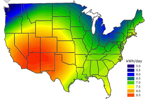
Using data from the annual simulations we created contour plot graphic representations of the estimated PV power produced throughout the U.S. The resulting performance contours are shown in Figure 1. Note that daily average PV power production varies from 5.5 - 9.0 kWh around the U.S. with best performance in the western states. The lowest levels are seen in the Pacific Northwest although the data show PV has good performance levels across most of the nation. Similarly, Figures 2 and 3 show the percentages of annual electricity and total energy cost requirements for the ZEH home met by the generic 2 kW rooftop PV system. Note that even a modestly sized 2 kW PV system will provide 48% or more of electrical energy requirements for the ZEH home anywhere in the U.S. and 25 - 70% of total energy costs outside of Alaska.

Figure 1. Average Daily Electricity Production (kWh/day) from a 2 kW Rooftop PV System

USA Map of Electricity Production
Color Graph

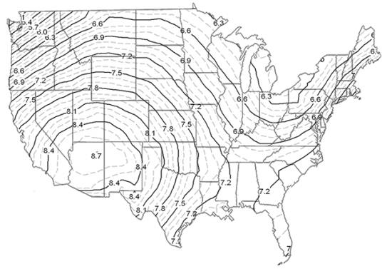
Figure 2. Percentage of Annual Electricity Requirements for ZEH
Provided by a 2 kW Rooftop PV system

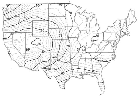
USA Map of Electric Requirement Percentages
Color Graph

Figure 3. Percentage of Annual Total Energy Costs for ZEH Offset by a 2 kW Rooftop PV System

USA Map of Energy Costs Percentages

Color Graph

Conclusions

We performed annual simulations for 236 TMY2 data locations throughout the United States on two highly-efficient one-story 3-bedroom homes with a generic grid-tied solar electric 2kW PV system. These annual simulations show how potential annual solar electric power generation (kWh) and potential energy savings from PV power vary geographically around the U.S. This gives designers and builders in a specific region an indication of their expected PV performance. We found that even a modestly sized 2 kW PV system will provide 48% or more of electrical energy requirements for a super efficient home in the continental U.S. and 25 - 70% of total energy costs (except Alaska). Making key efficiency improvements from a very-efficient home to a super-efficient home permits the fraction of the home’s total energy cost met by a 2kW PV system to increase from 27 to 37%, on average.

Furthermore, the same two generic prototypes were used in all locations for this analysis to show a conservative case. Better results could be accomplished by customizing the efficiency components of the home to fit that particular location. Future evaluations might consider the best ZEH designs by climate including cost information.

Acknowledgements

We gratefully acknowledge support of this analysis effort from the U.S. Department of Energy’s Building America Program. Thanks also to Zeke Yewdall for coding the PVFORM simulation and to Brian Hanson for implementing the necessary features into the simulation.

References

Balcomb, J.D., “Conservation and Solar: Working Together,” Proceedings of the 5 th National Passive Solar Conference, Amherst, MA, October, 1980.

Fuerlein, B.S., Chandra, S., Beal, D., Parker, D.S., and Vieira, R.K., “Evaluation of EnergyGauge USA®, a Residential Energy Design Software, Against Monitored Data,” Proceedings of the ACEEE 2000 Summer Study on Energy Efficiency in Buildings, Pacific Grove, CA, September 2000.

Lawrence Berkeley Laboratory, DOE - 2 Reference Manual, Building Energy Simulation Group, Applied Science Division LBL-8706, Rev. 2, Berkeley, CA, May, 1984

Marion, W., Urban, K., User’s Manual for TMY2s Typical Meteorological Years, Golden, CO, National Renewable Energy Laboratory, June 1995.

Menicucci, D.F., Fernandez, J.P., User’s Manual for PVFORM: A Photovoltaic System Simulation Program For Stand-Alone and Grid-Interactive Applications, Albuquerque, NM, Sandia National Laboratories, June 1994

Parker, D.S., Dunlop, J.P., 1994. “Solar Photovoltaic Air Conditioning of Residential Buildings,” 1994 Summer Study on Energy Efficiency in Buildings, Vol.3, p.188, American Council for an Energy Efficient Economy, Washington, D.C.

Parker, D.S., Dunlop, J.P., Barkaszi, S.F., Sherwin, J.R., Anello, M.T., and Sonne, J.K. “Towards Zero Energy Demand: Evaluation of Super Efficient Building Technology with Photovoltaic Power for New Residential Housing,” Proceeding of the ACEEE 2000 Summer Study on Energy Efficiency in Buildings, American Council for an Energy Efficient Economy, Washington, DC, Vol.1, p. 214, September 2000