

Reference Publication: Parker, D. S., "Research Highlights from a Large Scale Residential Monitoring Study in a Hot Climate." Proceeding of International Symposium on Highly Efficient Use of Energy and Reduction of its Environmental Impact, pp. 108-116, Japan Society for the Promotion of Science Research for the Future Program, JPS-RFTF97P01002, Osaka, Japan, January 2002. (Also published as FSEC-PF369-02, Florida Solar Energy Center, Cocoa, FL.) Disclaimer: The views and opinions expressed in this article are solely those of the authors and are not intended to represent the views and opinions of the Florida Solar Energy Center. |
Research Highlights From A Large Scale Residential Monitoring Study In A Hot Climate
Danny S. Parker
Florida
Solar Energy Center (FSEC)
FSEC-PF-369-02
Introduction
A load research project by a large utility has monitored 204 residences in Central Florida, collecting detailed electricity end-use load data. In each home, 15-minute electric demand data is obtained on total electric power, space heating, cooling, water heating, dryers, cooking and pool energy use. Interior and exterior temperatures were also recorded. This is similar to other detailed end-use data monitored in the U.S. Pacific Northwest in the ELCAP project (Pratt et al., 1989) and the PG&E Appliance Metering Project (Brodsky and McNicoll, 1987). However these data are of a more recent vintage and from a cooling dominated climate.
The homes represent a statistically drawn sample using end-use metering to identify ways in which the residential peak load might be reduced within its load management as well as to obtain improved appliance energy consumption indexes and load profiles. The extent of the collected data (100 million data points) provides an extremely rich data source for evaluating energy efficiency improvement potential of homes in hot climates. This paper highlights influences and findings.
Total and Other Electricity Consumption
Total electricity use was metered in all homes by monitoring incoming electrical service. Major end-uses were also recorded in each home on a 15-minute basis. These included space heating, cooling, water heating and either pool, dryer or range. We derived "other" electricity consumption by subtracting all the sub-metered end uses from total.
The total average annual electrical loads in the sample was 17,130 kWh. Other electricity consumption is large in magnitude within the homes. For homes where there was no non-metered pool, dryer or range, "other" averaged 5,730 kWh/year. Of this, space cooling averaged 5,650 kWh, space heating 1,070 kWh and water heating 2,240 kWh. Figure 1 below shows the relative fraction of each measured end-use.

Figure 1. Percentage of measured electricity
consumption
by end-use in pure sample (n=171).
Note that "other" is larger than any individually identified loads. Figure 2 shows the seasonality of total loads by month. A large transition to cooling takes place between March and May.
Figure 2. Seasonal load profiles of total power by time-of-day (n=171).
Space Heating Energy Use
The magnitude of residential space heating in Central Florida is small relative to more temperate climates. Since Florida's "winter" temperatures are often very close to the desirable interior thermostat setting, residential heating loads vary dependent on weather.
Figure 3 clearly shows the impact of weather comparing outdoor temperature against measured space conditioning loads over the entire year showing both heating and cooling.
Figure 3. Comparison of average outdoor temperature with space conditioning load over the entire year.
Florida's winters are exceedingly mild with very short cold snaps that feature intense electric demand for very short periods. These loads are very disadvantageous to serve as they have very short duration with the peak generation capacity unneeded for much of the year.
Heating System Types
Within the sample there were some 170 sites which were classified within the audit in terms of heating system type. Heat pumps were the most common heating system type, comprising 56% of the sample. Electric resistance strip heat was the next most common type at 33%. Natural gas and fuel oil heating comprised 8% and 2% of the sample, respectively. Three sites (2%) of the sample had "other" heating which were wood heat, portable space heaters and resistance heating on window air conditioners.
The reason heating and cooling degree days are commonly computed at a 65oF base is clearly indicated in Figure 4 which plots the 15-minute average heating and cooling varied over the year in the residential monitoring sample.
Figure 4. Measured average 15-minute space conditioning electric demand for all customers in the monitoring study against the outdoor temperature for the entire year of 1999. The 33,000 data points plotted are the average of more than 22 million collected over the course of the year.
Note how cooling ceases by 65oF and heating begins. The plot also shows why the utility is peak in winter. Although there are fewer hours in the heating domain, the maximum loads for space conditioning are almost 1 kW greater per household. For all of the heating analysis, we used all hours where the outdoor temperature was less than 65oF.
Space Heating Energy Consumption
Space heating energy use was recorded for each site and then averaged into the mean space heat across the residential sample. Since some cooling occurred at a number of sites during the period, an outdoor air temperature of 18.3oC was used as the dividing line between heating and cooling. As shown in Figure 5, the outdoor temperature does remarkably well describing when the average home ceases to require space heat.
Figure 5. Measured average heating load prediction for all of 1999.
However, the same trend shows that the demand for space heat is non-linear. It is quite steep from 0 to 10 degrees, but becomes flat and nearly asymptotic as 18oC is approached.
The regression function is superimposed on the plot. Much of the remaining scatter is explained by systematic differences with time of day. For instance, much of the data higher than the regression line is during nighttime hours. This suggests a non-temperature time-related component of space heat - likely solar gains.
The average measured space heat for all sites for the year of 1999 was 1,054 kWh but ranged from a low of 27 kWh to a high of 4,113 kWh. Figure 6 shows a histogram of measured space heating energy use.
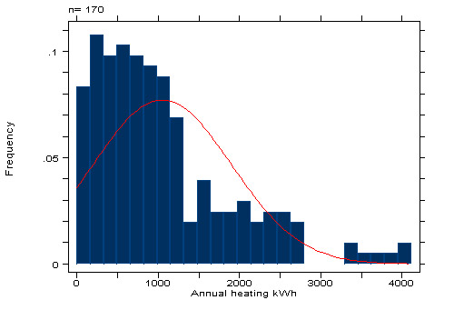
Figure 6. Histogram of January through December 1999 space heating.
The low consumption level was at Site 104 where the occupant allowed wide indoor temperature swings without space heat. The highest space heat consumer was Site 138 where strip heat is used and the occupants claim a desirable winter heating set point of 26oC. Auditors also observed evidence of significant duct leakage at this site.
Project summary statistics on space heating revealed several findings which fit expectations:
- Heat pumps reduce both energy consumption and peak demand
- Larger homes and older homes have greater energy use and demand
- Added ceiling and wall insulation show lower use and demand
- Homes with interior air handlers had lower demand
- Large expanses of single pane glass are associated with increased peak demand
- Installed heating system capacity is strongly associated with peak demand
The increased consumption of larger homes and less well-insulated is readily explained by heat transfer theory. The elevated demand of older homes likely arises from the confounding influences of greater saturation of electric resistance heating and lower insulation. The association of installed electrical capacity of space heating systems to peak demand is could be advantageously addressed within utility new homes program through a policy to size equipment.
Space Cooling Energy Consumption
As with heating, space cooling energy use was recorded for each site and then averaged into the mean space cooling across the residential sample. As shown in Figure 7, space cooling rises with outdoor temperature. However, demand for space cooling is also non-linear.
Figure 7. Plot of average cooling demand with outdoor temperature.
It is quite steep from 29 to 35 degrees, but becomes flat and nearly asymptotic as 18oC is approached.
The super-imposed function can be used with simple weather data to predict typical household cooling loads. The quadratic regression predicts an average measured space cooling of 5,557 kWh when used against the hourly temperature from April - October. On this basis, the estimate for annual space cooling (January 1 - December 31st) is 6,421 kWh. This shows that 90% of annual space cooling energy use is concentrated in the seven month period from April - October.
As with heating, much of the scatter is explained by systematic differences with time of day. For instance, much of the data is lower than the regression line is during nighttime hours. Much of the data is higher during the afternoon period. This suggests a non-temperature related component of space cooling - likely solar gains and thermal storage within the residential homes.
Figure 8 shows the end-use load source components on the peak cooling day of August 30, 1999.
Figure 8. End-use demand components on summer peak day (August 30, 1999).
The observation is the overwhelming dominance of space cooling on the load profile. Water heating is the second largest load except in homes which have pools (24% of the sample homes have them). The "other" category is large size as it includes refrigeration (~0.2 kW), plug loads and lighting. The later end-use is clearly seen at its maximum at 9 PM. Total electric demand for the one hour peak period from 4 -5 PM EST averaged 4.18 kW in the 169 sites in the base sample.
The average measured space cooling for all 169 FPC sites in the base sample from April through October of 1999 was 5,695 kWh. However, consumption varied by more than an order of magnitude, ranging from a low of 525 kWh to a high of 12,778 kWh. Figure 9 shows the frequency distribution of measured cooling energy use.
Figure 9. Frequency distribution of measured cooling energy use. A normal curve is superimposed.
The low consumption level was at Site 22 where the house was unoccupied for most of the summer season; the lowest occupied site was Site 114 (594 kWh) where the retired occupant is very frugal with operation of the air conditioning system. The highest space cooling consumer was Site 26 (12,778 kWh) a 200 m2 home where the occupants claim to maintain 22oC all season, the ceiling insulation is poor, a dark roof produces high attic temperatures and a relatively new 3.5-ton air conditioner is ill-matched to an old air handler.
Although there are a number of secondary factors, the data suggest that air conditioner size and thermostat setting are the fundamental driving forces in determining cooling energy use and peak demand in single-family. Key findings from the statistical and regression analysis:
Critical Parameters:
- Air conditioner size and maximum kW is a primary determinant of energy use peak demand. This was true even when accounting for floor area.
- Thermostat setting is a very large influence. Annual cooling energy use increases by about 7% for every degree that the interior temperature was lower.
Factors Increasing AC energy and demand
- Larger homes with greater conditioned floor area.
- Homes with fireplaces (likely due to increased air infiltration)
Factor Reducing AC energy and demand
- Higher levels of ceiling insulation
- Lower attic air temperatures produced by light colored roofs, tile roofs and shading
Factors Reducing AC peak demand
- Interior duct systems exerted a large influence
- Double-pane insulated glass
- West side exterior house landscape shading
- Homes exclusively using window unit air conditioners
- Concrete block construction vs. frame construction
Associated with the above factors (primary carriers):
- Two-story homes are larger with greater installed AC capacity
- Older houses are less well insulated, often with lower efficiency equipment
Hot Water Electric Demand and Consumption
The majority (150) of the water heating systems in the project were of the conventional electric resistance storage type. Eighteen of the monitored homes have natural gas or propane water heat and have no electric demand. Twenty (10%) of water heaters in the monitoring project have connected heat recovery units. There are also four operating solar water heating systems. There is also one tank-less water heater (Site 18). Eighty percent of water heaters were located in unconditioned spaces - primarily in garages. The rest were located inside the conditioned zone.
The water heating loads in Florida are somewhat lower than commonly supposed. Part of this is due to the advent of low hot water using appliances and showerheads (EPRI, 1997). Another part of the low consumption comes from occupancy and warmer water temperatures; some homes (e.g. Site 50) were unoccupied during much of the study while (e.g. Site 22) turned off the water heater breaker when away from home for extended periods.
As expected, the summary statistics on hot water heating showed that occupancy has the strongest influence on variation in energy consumption. Average annual electricity consumption for electric resistance systems averaged 6.4 kWh/day or 2,325 kWh/year. Consumption varied considerably by occupancy. Average number of occupants was 2.81, but two occupants was the most common household number. Figure 10 shows a variable width box plot of DHW electricity use against household occupants.
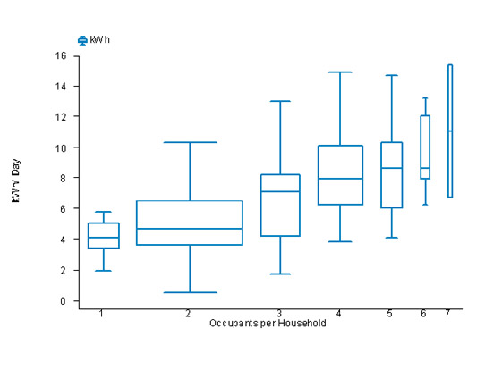
Figure 10. Box plot of daily DHW electricity variation with household size. Center line of the box is median, box top and bottom are inner quartile range. Box width is proportional to sample size.
Beyond household characteristics, the water heating data revealed that hot water tanks with external insulation wraps and those located within the conditioned space showed lower winter utility coincident peak demand (16% and 10% respectively).
Figure 11 shows a histogram of the frequency distribution of measured hot water energy use.
Figure
11. Histogram of daily hot water electricity.
Day of Week Variation in DHW Loads
Figure 12 shows the impact of the day of the week on average measured water heating electrical loads over the entire year of 1999.
Figure 12. DHW electricity use and peak demand by day
of week.
The brown bars show the impact of day of the week on daily average consumption (kWh/day) while the connected superimposed line shows the impact on the average DHW electrical load between 7 and 8 AM in the morning. This is important since it is generally the time of the daily winter morning system peak demand.
Weekday
water heating energy use is similar. Mondays have the
greatest consumption and Friday are a bit lower, perhaps
due to early weekends. However, weekend days clearly
show increased hot water energy consumption (greater
occupancy), but generally peaking at a later time of
day (households sleeping in). Sunday shows the greatest
difference in consumption and 8 AM peak demand from the
other days of the week.
Seasonality of Water Heating
Loads
Although water heating is not totally dominated by weather like space heating and cooling, these loads are still sensitive to temperature conditions. Figure 13 shows how daily average hot water energy use varied in the sample by the daily average air temperature measured in the project.
Figure 13. Impact of air temperature on daily average DHW use.
Although, there is considerable scatter. A simple linear regression plotted explains 58% of the variation in the day-to-day hot water energy consumption. Moreover, including a dummy variable for weekends does little for the regression. DHW use is just slightly higher on weekends and the demand profile differs, however this is not nearly as great as that of temperature.
There are several reasons for this influence:
- Tap water temperatures vary seasonally by about 8oC in Central Florida as seen in Figure 14. Although the annual inlet water temperature averages 24oC, this varies to a high of about 27.2oC in September to a low of 19.4oC in February as ground water piping is affected by weather conditions.
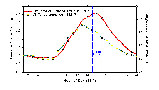
Figure 14. Measured variation of mains water temperature over the year in Central Florida.
- Greater standby losses. Colder air temperatures lead to greater standby losses for storage tank types - particularly those in garage locations.
- High hot water use. Colder air temperatures lead to greater hot water use as household members take longer showers to warm up and use more hot water within the mix to achieve the preferred water temperature. This has been observed in previous monitoring projects where hot water consumption increased by 15-20% from summer to winter (Merrigan and Parker, 1991; Brecker and Stogsdill, 1990).
The summer data shows even greater weather related impact for water heating. As shown in Figure 15, water heating loads are greatest during the colder months.
Figure 15. Measured DHW load profiles by month.
April clearly shows the shift in timing of water heating load imposed by Daylight Savings Time. The later spring and summer months show progressively lower water heating loads.
Water Heating System Type
We examined how water heating system type influenced electric demand and energy use. Some 10% of the sample had heat recovery units which scavenge heat from the air conditioning system to heat hot water. Four homes had operating solar water heating systems. Figures 16 and 17 display performance characteristics of these water heating systems.
Figure 16. Measured DHW load profiles by month.
Figure 17. Measured January DHW load profiles by system type.
As expected, the average demand profile in July shows that HRU water heater used less electricity than the electric resistance group in all hours. The electric resistance water heaters use about 5 kWh per day as opposed to 2.3 kWh for the HRU systems. The demand reduction from 4 - 5 PM is only 100 Watts, however. The savings in daily water heating energy use is 2.7 kWh or approximately a 54% reduction in water heating energy.
The situation for winter months shows less advantage. First, the HRU systems used 34% less energy. They also reduce electric demand slightly in winter compared to their electric resistance counterparts. The demand difference between the two systems from 7- 8 AM during January was approximately 110 Watts or about a 22% reduction in utility winter coincident morning demand.
Over the one year period, the average consumption for electric resistance water heating systems was 6.37 kWh/day as opposed to 4.63 kWh/Day for the HRU systems (suggesting annual DHW energy use of 2325 and 1689 kWh, respectively). This is a similar level of performance that was observed in another comparative project in which HRUs and electric resistance systems were metered (Merrigan, 1983).
The four operating solar water heating systems showed large reductions in demand as well as energy. The reduction in annual energy use was 61% against electric resistance systems. This indicated an annual average electrical reduction of 1,420 kWh/year. Peak reductions were approximately 0.31 kW in winter and 0.14 kW in summer.
Other End Uses
We briefly summarize collected data on a number of other end-uses: cooking, clothes dryers, swimming pool pumps and even spas. Of these, swimming pool pumps were largest in measured end use - averaging 4,200 kWh/year in the 24% of homes which possessed them. Electrically heated spas or Jacuzzis were in 7% of homes in the sample. They showed an average electrical consumption of 2,150 kWh. Figure 18 shows how the swimming pool pump electrical demand profile varied over the year.
Figure 18. Time of day average pool electrical demand by month.
It is strongly a daytime load and thus may be an ideal candidate to be offset with solar electricity.
Clothes dryers were the next largest end use, representing a consumption of 885 kWh/year in the 90% of homes which had them. Figure 19 shows their broad load-demand profile.
Figure 19. Monthly demand profile for clothes dryer.
The energy use of electric ovens and ranges (93% of homes) was surprisingly low, likely reflecting the increasing prevalence for dining out and non-cooked breakfast foods in the United States. Measured cooking energy use averaged only about 300 kWh/year with the evening-weighted load demand profile shown in Figure 20.

Figure 20. Monthly demand profiles for electric range/oven.
Growth in Appliance Consumption
Our analysis allowed us to examine how lighting, minor appliances and other plug loads influence electricity use and demand. This was done by subtracting measured end-use loads from totals. Figure 21 shows how "other" appliance energy use and demand varies over the year.
Figure 21. Variation in other electricity use by time of day.
"Other" in this case consists of lighting, refrigerator and plug loads.
Figure 22. Average "other" electricity use in FPC homes over 1999.
The time-series plot in Figure 22 shows how other electrical demand varies for all of the sites in the statistical sample over the year of 1999. The green symbols show the 15-minute average power demand of "other." This represents an average of the 170 sites.
The red line in the above plot represents the average demand by day. There was a pronounced relationship by time of year and by time of day. Obviously, much of the observed variation has to do with the daily cycle. The pronounced impact of holiday lighting is clearly seen. The minimum in the summer loads rises, likely due to greater refrigeration and ceiling fan use.
There was a slow, but steady increase in "other" over the year. The graph shows that average daily appliance energy use (averaged for all sites with 15-minute data) grows somewhat over the course of the year; note that both the peak values are higher and the lows are lower in the cooler months, while the summer consumption varies less. A linear regression on the data, excluding the bias from the winter holiday reveals that:
kW = 0.668 + 0.000342 (Julian Date)
The t-statistic for julian date was 36.2, indicating very high statistical significance that appliance use was growing over the period. The relationship would indicate that "other" appliance consumption increased by an average of 8.2 Wh/day over the period. The relationship estimates that "other" appliance energy use grew by about 17% over the period.
Likely reasons for the growth is increasing saturation of personal computers (PCs) and other plug loads using power packs (phones, cellular phone chargers, etc.) as well as a progressive economy. We also know from the DOE Residential Energy Consumption Survey data (EIA, 1995) that home computers are the fastest growing home appliance segment. A PC and monitor draw about 150 watts when operating so that 3 hours of household use per day would add about half a kWh in daily energy use. The saturation of personal computers in the FPC appliance audit was 72% in 1999.
Conclusions
The project has identified a number of influences on energy use and demand that are not commonly described. The results show that building energy monitoring can be a powerful means to learn new methods to control the growth in residential electric demand.
Acknowledgment
Special thanks to John Masiello at the Florida Power Corporation (FPC) for releasing parts of this otherwise proprietary study. Matt Bouchelle at FPC; Mike Anello and Katie Richards at FSEC were also instrumental in the data analysis.
References
Brecker, B.R. and Stogsdill, D. E., 1990. "A Domestic Hot Water Use Database," ASHRAE Journal, September, Atlanta, GA
Brodsky, J.B. and McNicoll, S.E., 1987. "Pacific Gas and Electric Company Residential Appliance Load Study, 1985-1986," Pacific Gas and Electric Company, Berkely, CA.
EIA, 1995. Housing Characteristics 1993, DOE/EIA-0314, Residential Energy Consumption Survey, Energy Information Administration, Washington, DC, June, 1995.
EPRI, 1997. "EPRI Hot Water Consumption Study Refutes Common Assumptions," Electric Water Heating News, EPRI, Palo Alto, CA, Summer.
Merrigan, T. and Parker, D., 1991. "Electrical Use, Efficiency, and Peak Demand of Electric Resistance, Heat Pump, Desuperheater, and Solar Hot Water Heating Systems," Proceedings of the 1990 Summer Study on Energy Efficiency in Buildings, Vol. 9, p. 221, American Council for an Energy Efficient Economy, Washington D.C.
Merrigan, T., 1983. Residential Conservation Demonstration: Domestic Hot Water, Final Report, FSEC-CR-90-83, Florida Solar Energy Center, Cocoa, FL.
Pratt,
R.G., et al., 1989. "Description of Electric Energy
Use in Single-Family Residences in the Pacific Northwest,"
End-Use Load and Consumer Assessment Program (ELCAP), Pacific
Northwest Laboratory, DOE/BP-13795-21, Richland, WA, April
1989.
Presented
at:
The International Symposium on Highly Effective Use of Energy and Reduction of its Environmental Impact. Osaka, Japan, January 22-23, 2002
© 2007-2014 University of Central Florida. The Florida Solar Energy Center (FSEC)
is a research institute of the
University of Central Florida.
For more information about FSEC, please contact us or learn more about us.
Find us on Facebook!