| Consumer | Education | Research |

| Testing & Certification |

Reference Publication: Bouchelle, M P, D S Parker, M T Anello, and K M Richardson , 2000. "Factors Influencing Space Heat and Heat Pump Efficiency from a Large-Scale Residential Monitoring Study." Proceedings of 2000 Summer Study on Energy Efficiency in Buildings, American Council for an Energy-Efficient Economy, 1001 Connecticut Avenue, Washington, DC. Disclaimer: The views and opinions expressed in this article are solely those of the authors and are not intended to represent the views and opinions of the Florida Solar Energy Center.

Factors Influencing Space Heat and Heat Pump Efficiency from a Large-Scale Residential Monitoring Study

Danny S. Parker
Michael T. Anello
Katie M. Richardson
Florida Solar Energy Center (FSEC)

and

Matthew P. Bouchelle
Florida Power Corporation

FSEC-PF-362-01

Abstract

Since Florida utilities often experience their system peak during the state's few cold mornings, understanding influences on space heat performance is important to controlling demand. Analysis of heat pump impacts on system load in a large scale monitoring study have shown large levels of strip heat being used during the winter morning peak. The implied coefficient of performance of heat pumps during the system peak hour was only 1.30. Also, analysis of the total seasonal space heat has shown that the implied Heating Season Performance Factor (HSPF) of heat pump homes is only 4.4 Btu/W rather than the 6-8 Btu/W commonly claimed. This paper describes reasons for the lower than anticipated levels of performance as well as other significant influences on space heating demand.


Introduction

A utility load research project by the Florida Power Corporation (FPC) is monitoring 200 residences in Central Florida. The homes represent a statistically drawn sample using end-use metering to answer specific load research questions. A prime objective of the monitoring is to identify ways in which the winter morning residential peak load might be reduced within its load management and DSM programs.

As with many utilities, FPC, through rebates, encourages the selection of heat pumps within its service territory as a means to reduce the magnitude of the winter morning heating peak. This objective has largely been realized. Within the statistical sample, 118 homes or 58% possess heat pumps, 32% had electric resistance systems and 9% used natural gas or oil furnaces. Thus, 64% of electric heating systems in the service territory are heat pumps. The expectation has been that the mild conditions of Florida's winter should allow heat pumps to operate under favorable conditions and provide lower peak demand than electric resistance systems.


Residential Heat Pumps

A residential heat pump takes low-temperature heat from an outdoor medium (such as air, ground, groundwater or surface water) and mechanically concentrates it to produce high temperature heat suitable for heating the interior of homes. Because most of the heat is moved (pumped) from the outdoor source to the indoor source, the amount of electricity required to deliver it is theoretically much less than using electric resistance heat directly.

Heat pumps were introduced to the home heating market in the 1950s, evolving originally from central air conditioners which featured a reversing valve and a few other factory components allowing the heat pumps to provide heat under mild weather conditions. Early models were plagued with reliability problems related to failed reversing valves, improperly operating compressors or frost build up on the evaporators. Performance under colder conditions was often poor due to reduced heating capacity at low outdoor temperatures. Comfort was another complaint with early systems due to "cold blow" where the air temperature delivered by the heat pump was much lower (typically 100 - 105^oF) compared with the 125 - 130^oF typically delivered by natural gas furnace systems.

Modern heat pump systems are much more reliable and have become exceedingly common in Sunbelt states. By far the most common types are air-to-air heat pumps which use outdoor air as the heat exchange medium. The problems with inadequate capacity and "cold blow" have been reduced by the addition of auxiliary resistance strip heat systems with a two-stage thermostat. As the indoor temperature drops, the first stage activates the heat pump; the second stage below it activates auxiliary strip heat. Under this regime, both the heat pump and the resistance heat operate together until the thermostat is satisfied.

The theoretical Carnot efficiency of heat pumps is greater than 2000%. Thus, the COP, or coefficient of performance, would indicate 20 times as much heat delivered as used. However, the practical efficiency of the best air-to-air heat pumps produce COPs of 3.0 or less. Because COP varies with the outdoor temperature, a heating season performance factor (HSPF) is determined which takes into account operation under varying outdoor temperatures as well as part load impacts (effects of running short cycles under mild conditions, coil defrost, etc.). HSPF is rendered as Btu/Watt so that typical values are on the order of 6.8 - 8 Btu/W.⁽¹⁾ Older systems may have HSPFs of 6 - 7 Btu/W.

In the past, utility DSM programs have strongly leaned on heat pumps to reduce winter peak coincident demands. Reductions in peak demand over the use of strip heat have often estimated savings of 50 - 70% even when allowance for supplemental strip heat use was made (AEC 1993). Unfortunately, most previous studies examining heat pump performance have ignored how operation and system related factors can influence field performance.


Empirical Tests of Heat Pump Performance

As heat pump technology re-emerged in the early 1970s, a number of evaluations were performed. Many laboratory studies were conducted under steady state conditions to evaluate impacts of defrost, crankcase heat and other influences (eg. Parker et al. 1977; Rettberg 1980).⁽²⁾ It has been long known that even with a constant thermostat setting and optimal system operation that as the building loads exceed the declining capacity of the heat pump with lower temperatures that the difference must be made up with resistance heat and this will impact overall efficiency (Reddy and Daniels 1992). However, few studies have examined how heat pumps operate in real homes where thermostat settings are altered, indoor coil air flow may be lower than expected and refrigerant charge may vary from an optimal configuration.

Many of the early investigations did show that heat pump performance was lower than would be expected by the procedures established to estimate HSPF. In a study for Louisiana Power and Light Company, Orth et al (1976) performed alternate day resistance heat measurements on two 1967 vintage heat pumps and found seasonal coefficient of performance (SCOP) measurements of 1.75 and 1.78 for the systems against the standard seasonal SCOP rating of 2.25 based on manufacturer's data. In the colder climate of New Jersey, Nicolich (1977) estimated the SCOP of a single heat pump to be 1.65 based on pre and post measurements. In the much colder climate of Ontario, Canada, 40 heat pumps were monitored in detail showing average SCOPs of 1.43 over the heating season from 1975-1977 (Miller and Jaster, 1985). Similarly, a large study by Carrier Corporation (Groff et al. 1978) showed average seasonal COP values of 1.2 to 1.61 in the Boston and Minneapolis climates.

However, even in moderate climates, performance may be less than anticipated. Four residences in Albuquerque, New Mexico had heat pump performance evaluated through alternate day resistance heat operation. This showed SCOPs averaging only 1.39 as opposed to the HSPF calculation which indicated a COP of 1.85. The study determined that homeowner operation of thermostats was largely responsible for the lower than expected savings. Another study in Knoxville, Tennessee of two heat pumps (Baxter 1981) yielded measured SCOPs of 1.58 and 1.99 respectively against calculated SCOPs of 1.99 and 2.61.

In summary, although there is justification for the DOE test procedures that predict heat pump seasonal performance (Miller and Jaster 1985), there is reason to suspect that the actual achieved seasonal COPs are significantly lower than suggested by HSPF values.


Thermostat Setback and Electrical Heating Systems

A number of studies stretching back to the early 1970s show that substantial energy savings can be achieved through the use of thermostat setbacks with heating systems (Nelson 1973; Pilati 1975). Both computer simulation as well as experimental testing has confirmed the savings of night setback of heating systems with constant capacity (Quentzel 1976). Measured seasonal energy savings are on the order of 10-15% - greater in milder climates. However, the same studies have highlighted the increase in morning heating pick-up load. Although this is unimportant for natural gas or oil furnaces, the same is not true for electric resistance forced air systems where utility peak coincident demand may be significantly elevated during the morning set-up period.

The impact of thermostat set back on energy savings with heat pump systems is much less clear. This is due to the fact that the thermal performance of the heat pump is not independent of the house heating load. The heating capacity of an air-to-air heat pump drops with lower outdoor temperature while the house thermal load increases. If the heat pump capacity drops below the building thermal load, the lower efficiency supplemental electric resistance heaters must make up the difference. This issue became evident in early test results from heat pumps in northern climates. However, an early hourly simulation analysis with a detailed heat pump model (Ellison 1977) revealed that while peak morning heating loads were increased by up to 100% (~4 kW for a three ton heat pump in Atlanta) during the morning pick-up hour, the homeowner would realize energy savings of 7 - 15% for a 60^oF setback and 10-18% for a 55^oF setback.

In spite of the simulation results, field information gathered by utilities in the cold winter of 1976-1977 suggested that setting back heat pump thermostats would lead to elevated consumption and greatly increased demand (Air Conditioning, Heating and Refrigeration News 1977). Contrasting the earlier ORNL analysis was another done by the Carrier Corporation (Bullock 1978). This study concluded that the savings from thermostat setback with heat pumps was modest (2 - 4%) or even negative, largely depending on the installed capacity of the strip heaters. Since resistance heat elements are often installed in 5 kW increments and are typically larger than those assumed in the ORNL evaluation, this becomes a significant limitation in its conclusions. In contrast, the Carrier study concluded that a setback more than a couple of degrees (^oF) with a heat pump will lead to only small seasonal heat energy savings while producing very high morning power demand.

For instance the Carrier evaluation for a mild 44^oF day in Minneapolis, similar to the coldest winter day in Orlando, showed a daily heating energy consumption for a typical home of 22.8 kWh for no setback with approximately 2 kW of demand at 7 AM. However, a 10^oF setback with morning setup at 7 AM, lead to a daily reduction in heating energy of 2.4 kWh (10%), but with an increase of total electric demand of 9 kW!⁽³⁾ The study concluded that setbacks should not be used with heat pumps until adaptive thermostat technology was fully developed.

Florida's Mild Winter

Florida's warm winters would seem ideal for heat pump application. Florida weather is not commonly thought of as possessing a winter. While not having a long heating season, it does have short and sporadic space heating which is very much concentrated during a few cold mornings. The magnitude of residential space heating in Central Florida is small relative to more temperate climates. Since Florida's "winter" temperatures are often very close to the desirable interior thermostat setting, residential heating loads are very dependent on weather.

The first three winter months of 1999 during which the data were collected were mild (Table 1). The average temperatures were about two degrees warmer than the 30 year normals, although the extreme minimums and maximums were in line with the typical expectation. The heating degree days, which may approximate energy use, show that while cooling degree days were similar to the normals (84%), heating degree days were under 60% of the thirty year normals.

Table 1. Comparison of 1999 Winter Weather with 30 Year Normals.

Month of Year	Average Dry bulb ( + F)	Maximum (Julian Date)	Minimum (Julian Date)	Heating/Cooling Degree Days (+ Normal)
January	63.9 (+ 4.2)	86 (023)	31 (006)	109 (-125) | 82 (+12)
February	64.0 (+ 2.8)	84 (049)	39 (055)	92 (-72) | 69 (+11)
March	64.6 (- 2.1)	84 (088)	40 (064)	61 (-4) | 54 (-63)
Period	64.2 (+1.7)	86 (023)	31 (006)	262 (-201) | 205 (-40)
30 Yr Norm	62.5	87.4	32.1	463 | 245

A unique part of the FPC project is that outdoor temperatures are being collected at each of the 204 sites. This allows analysis of how temperatures around the homes vary by region and local microclimate. The temperature data collected in the project mirrored weather data taken at Orlando International Airport, although there are greater extremes with respect to individual sites. The 15-minute average air temperature and space conditioning demand for all sites for January - March of 1999 are graphically illustrated in Figure 1.

Figure 1. Comparison of average outdoor temperature with space conditioning loads.

The key evidence seen in Figure 1 is that Florida's winters are exceedingly mild with very short cold snaps that feature intense electric demand for very short periods. These loads are very disadvantageous to serve as they have very short duration with the peak generation capacity unneeded for much of the year. Evidence of space cooling is even seen in the data for the warmer period around January 23^rd.

An important influence is seen in Figure 2 which displays a histogram of heating degree days at a 55^oF base when plotted against time for Central Florida weather over the winter of 1999.

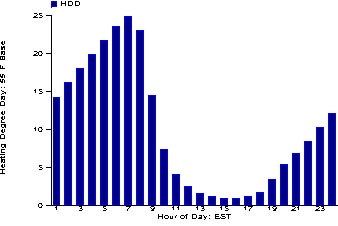
Figure 2. Frequency distribution of space heating degree days by the time-of-day for winter 1999.

Note the concentration of heating in the morning hours between 5 and 8 AM when nighttime thermostat set-backs are often setup. For heat pumps, this means that much of the heating occurs during periods which electric resistance heat will be required if thermostats are adjusted.


Space Heating Energy Use

Space heating energy use was recorded for each site and then averaged into the mean space heat across the residential sample. Since some cooling occurred at a number of sites during the period, an outdoor air temperature of 65^oF was used as the dividing line between heating and cooling. As shown in Figure 3, the outdoor temperature does remarkably well describing when the average customer ceases to require space heat.

Figure 3. Relationship of average outdoor temperature to measured 15-minute space heat demand

However, the same trend shows that the demand for space heat is non-linear. It is quite steep from 30 to 50 degrees, but becomes flat and nearly asymptotic as 65^oF is approached. A regression based on ambient air temperature (T_amb) below 65^oF adequately predicted average hourly space heating demand for the overall sample:

Heat kW = 16.228 - 0.502 (t_amb) +0.00389 (t_amb²)
R² = 0.87

The function is superimposed on the plot in Figure 3. Much of the remaining scatter is explained by systematic differences with time of day. For instance, much of the data higher than the regression line is during nighttime hours. Much of data is lower during the afternoon period. This suggests a non-temperature related component of space heat - likely solar gains. The function can be used with simple weather data to predict typical household heating loads.

When applied to TMY weather data for Orlando for the "typical" January - March, the regression predicts 658 kWh. When applied to the entire year of TMY data including November and December, it predicts the typical Central Florida residential site would have used 1092 kWh for space heat under average weather conditions. The regression also predicts that for an hour when the outside air temperature is 40^oF the per site heating demand the utility service territory will average 2.27 kW, when the outside air temperature is 30^oF, it will average 4.41 kW.

Space heat was estimated for each site based on recorded electricity use on the space heat circuits when the outdoor air temperature was lower than 65^oF. Gas heated sites were not included in the evaluation. The average measured space heat for all FPC sites from January through March of 1999 was 616 kWh. However, consumption varied by two orders of magnitude, ranging from a low of 22 kWh to a high of 2,283 kWh. Figure 4 shows a histogram of the frequency distribution of measured space heat energy use.

Figure 4. Histogram of Jan-Mar space heating.

The low consumption level was at Site 104 where the occupant allowed wide indoor temperature swings without space heat. On the coldest morning of January 6^th, the household allowed the interior to reach 60^oF with no space heat. The highest space heat consumer was Site 138 where strip heat is used and the occupants claim a desirable winter heating set point of 80^oF. Auditors also observed evidence of significant duct leakage at this site. The summary statistics on space heating in Table 2 reveal several findings:

• Heat pumps reduce both energy and peak demand, but not by half
• Larger homes and older homes have greater energy use and demand
• Added ceiling and wall insulation show lower use and demand
• Homes with interior air handlers had much lower demand
• Large areas of single pane glass are associated with increased peak demand
• Better insulated glass is correlated with lower peak demand
• Installed heating system capacity is strongly associated with peak demand

Table 2. Impact of Selected Characteristics on Space Heat Energy Use and Demand.

Characteristics		Heat kWh	n	kW	n
Vintage:	< 1980 > 1980	733 580*	81 87	3.157 2.505*	70 87
Stories:	One Two	648 626	176 9	2.841 2.058	148 9
Floor Area:	< 1600 ft2 > 1600 ft2	588* 715	99 86	2.540* 3.105	86 71
Heating System:	Electric Resistance Heat Pump Gas/Oil Portable Heaters	757** 589*134* 464	68 11819 4	3.337** 2.558*0.904* 1.078	60 9816 4
Installed kW:	< 9 kW > 9 kW	508* 781	91 94	2.264* 3.321	78 79
Jan. 5th Interior Temp.:	< 70oF >70oF	557 739**	93 95	2.358 3.382**	93 67
Setback w/Setup:	< 1oF > 1oF	685 587*	113 72	2.572 3.353**	112 45
Fireplace:	Yes No	722 612	59 126	3.071 2.678	47 110
Air Handler Location:	Attic Interior Garage	678 638 680	49 54 79	2.680 2.222* 3.292**	42 45 67
Ceiling Insulation (R-value):	< 20 hr · ft2 F/Btu > 20 hr · ft2 F/Btu	699 602*	87 107	3.026 2.525*	75 88
Wall Type:	Block Frame Mixed	662 684 576	126 21 38	2.746 3.096 2.791	106 18 33
Wall Insulation (R-value):	< 4 hr · ft2 F/Btu > 4 hr · ft2 F/Btu	708 619	59 126	3.139 2.621	53 104
Glass Conductance:	> 200 Btuh/oF < 200 Btuh/oF	681 588*	117 68	3.068 2.368*	96 61
Programmable Thermostat:	Yes No	675 656	41 144	2.662 2.830	32 125

* Significantly lower at a 90% level
** Significantly higher at a 90% level

The increased consumption of larger homes and expanses of single glass is readily explained by heat transfer theory. In fact, all the building surface areas divided by the R-values of the audited components were significant in their impact on measured space heating and demand. On the other hand, the elevated demand of older homes likely arises from the confounding influences of greater saturation of electric resistance heating and lower insulation.

A key finding, however, is the ratio of heating energy use in electric resistance homes (757 kWh) to that in heat pump homes (589 kWh). The implied seasonal heat pump coefficient of performance is only 1.29 with a high degree of significance. The differences in the peak demand of the two systems (779 W or 23%) was even less pronounced - and much less than the 50% or greater reduction that might be expected. The implied peak performance of heat pumps compared with electric resistance systems was 1.30.


Heating Thermostat Behavior

One of the most interesting findings was the way in which thermostat settings influence energy use and demand. Occupant reported thermostat settings did not well characterize measured space heating consumption, although the recorded interior temperature showed strong correlation with space heating demand. For instance, the measured average interior temperature during a cold snap was significant not only at predicting the site peak demand the following morning, but also of characterizing space heating use over the entire winter season.

Also important was the measured "pickup" load on January 4^th - 5^th. This was estimated as the difference between the measured interior temperature at 8 AM on January 5^th from the recorded temperature four hours earlier at 4 AM. The "pickup" load is analogous to the thermostat setup during early morning hours after allowing it to drop during the evening.

Some 115 project homes had a less than 0.5^oF pickup. For the most part these homes had a relatively constant thermostat setting with a few allowing the temperature to fall throughout the night and depart during the morning hours without setting back the thermostat. In these homes, the average space heat demand between 7 and 8 AM was 2.33 kW (n=115).

A total of 48 households practiced a 'deep thermostat' setback during the evening hours with the temperature set up in the early morning hours. The average temperature recovery or "pickup load" between 4 and 8 AM was 3^oF. While these households did reduce their total space heating energy by about 14% (Figure 5), this practice dramatically increased space heat demand during the utility coincident period.

Figure 5. Influence of nighttime winter setback on peak demand: January 5, 1999.

The average hourly demand in this group of homes was 3.19 kW during the peak time frame. The difference in diversified demand (0.86 kW) was significant at the 99% confidence level. A third of the monitored sample use deep setback, suggesting that deep thermostat setbacks with a morning setup may be responsible for up to 300 MW in increased utility peak load.

To better understand this problem, it is useful to examine a heat pump case with strip heat demand. Figure 6 shows the heating demand profile at Site 2 on the coldest day of the year (January 5^th).

Figure 6. Measured heat pump operation at Site 2 - Jan 5, thermostats sets up temperature 2^oF at 7 a.m.

The programmable thermostat at this site raises its setting at 7 AM by 2^oF. This activates the strip heat for a single 15 minute cycle after which the strip drops off and the heat pump properly returns to compressor operation (~4 kW with air handler). Many sites showed similar behavior. With thermostat set-up with heat pumps, strip heat will be used on cold mornings.

Winter Peak Demand

The utility winter peak for 1999 occurred between 7 and 8 AM on January 6^th. The minimum temperature at the Orlando International Airport was 31^oF at 7 AM. Figure 7 shows that the total electric demand for a one hour period averaged 5.74 kW in the 114 all-electric non-load control sites with valid data (22 sites had missing data or were not yet on-line). The importance of the heating load to total peak demand is seen in the end-use component summary in Figure 7.

Figure 7. End-use load components during winter system peak hour.

Figure 8 shows a frequency distribution of hourly space heat demand for all sites on the morning of January 5^th, 1999.

Figure 8. Space heat demand histogram for all electric sites between 7-8 a.m. on Jan 5, 1999.

This was the coldest non-load controlled day. Although space heat demand averaged 3 kW between 7 and 8 AM, 20% of customers used no space heat at all, while some sites had demand as great as 12 kW.

The significance of heating system type on peak demand is seen from a segmentation of the data. Within the sample of 204 homes, 60% were heat pumps (the most common type), 33% were strip heat with the balance using natural gas, fuel oil or propane. Several homes (Sites 077, 161,166, 172, 175) had window units with either strip heat or a reversible heat pump. Sites 16, 19, and 201 have fuel oil heat. A number of houses (8%) also reported using either portable space heaters of either the electric or kerosene type.

Heat Pump Performance

On January 6^th, non-load controlled homes with heat pumps experienced an average total household electric demand of 5.11 kW during the peak hour as opposed to 6.63 kW in homes with electric resistance heating. As expected, homes using strip heat showed almost all of the activity on the air handler circuit (4.66 kW; n = 43). Surprisingly, however, the 68 homes with heat pumps showed a large amount of back-up strip heat on the air handler circuit (1.70 kW), averaging more than that recorded on the compressor side (1.61 kW). A significant number of homes with heat pumps showed coincident demand on the air handler side greater than 7 kW indicating that a large capacity of back-up strip heat is installed.

Three sites showed evidence of improper operation with emergency heat being commonly activated during morning heating. This may be due to misunderstanding about proper heat pump operation and/or choice of this mode due to insufficient recovery time or discomfort. Figure 9 illustrates improper heat pump operation at Site 99.

Figure 9. Use of strip heat at Site 99 on Jan 5, 1999 after a deep setback.

There were other physical problems in several sites which led to strip heat operation. Site 88 had a non-functional compressor and sites 55, 68, 102, and 117 had an improper thermostat installed so they operate as if they were a strip heat system.

More problematic, however, is the impact of thermostat setup on heat pump performance. When these are reset and cannot meet load, internal control logic on adaptive control type thermostats often activate emergency strip heat.⁽⁴⁾ Heat pumps controlled by conventional analog-type mercury-bulb bi-metal thermostats will be triggered into strip heat if the thermostat is adjusted more than 2^oF away from the current temperature. Since most set-backs and set-ups are more than 2^oF, strip heat will be required during the period subsequent to thermostat set-up. Also, some heat pumps feature a time delay which allows strip heat and the air handler fan to operate for some time after the thermostat has stopped calling for heat. Finally, misinformed or frustrated customers may activate "Emergency Heat" on the thermostat which moves the heat pump into directly strip heat mode.

Although homes with heat pumps used less heating energy during the monitoring period, the demand characteristics of these systems were disappointing when compared against electric resistance types. Figure 10 shows the average performance of these systems.

Figure 10. Heat pump compressor and strip heat electric demand and interior temperature in group of homes exhibiting good performance: Jan 5, 1999.

To further examine the issue, we segmented the performance of heat pump systems on the coldest non-load control day (January 5, 1999) by their relative strip heat use. Examining the performance plot for each individual system we found that 62 of 99 systems (63%) showed fair to good performance with large levels of compressor operation (27.1 kWh) and relatively little strip heat the air handler circuit (7.3 kWh).

By comparison, some 33 systems (33%) showed very high levels of strip heat consumption (36.4 kWh) compared with compressor (20.4 kWh). The averages for these systems are shown in Figure 11.

Figure 11. Heat pump compressor and strip heat electric demand and interior temperature in group of homes exhibiting poor performance: Jan 5, 1999.

Total space heating energy for the day varies significantly: 57 kWh for the group using considerable strip heat against 34 kWh for the group using mainly the heat pump compressor.

Even more revealing are the recorded average interior air temperatures in the two groups. Whereas the group with superior heat pump operation maintained more constant temperatures on average, the group with large levels of strip heat allowed large fluctuations from the evening to morning temperature, suggesting a greater degree of nighttime setback. In general the group practicing more even temperature control also achieved better comfort with lower total consumption. For instance, between 7 and 8 AM, the group with good heat pump operation showed a demand of 2.24 kW against 3.53 kW for the group with excessive strip heat use. At the same time, the households with better heat pump operation maintained 70.3^oF inside against the 69.0^oF in the homes using considerable strip heat. Although thermostat setback (strip heat) is a large factor explaining poor performance, there are other reasons. Examination of data from individual sites suggested resistive coil defrosting was responsible for a portion of the shortfall.

Also, previous assessments have shown that low air handler airflow can significantly reduce heat pump capacity with all of 27 audited forced air installations exhibiting this problem (Parker, et al., 1997). Improper refrigerant charge has also been identified as a large issue in many heat pump installations which adversely impacts performance (Proctor, 1997; Blasnik et al., 1996). Finally, there are the issues of installation of non-heat pump thermostats on heat pump systems as well as inappropriate use of "emergency heat." Such factors reduce the efficiency of heat pumps relative to electric resistance systems. Our findings suggest several opportunities for improving heat pump performance:

• Load control could concentrate on interrupting strip heat on homes with heat pumps so that they may not be operated during the control window.
• Adaptive recovery thermostats to reduce the frequency of strip heat through slowly staged thermostat set-ups.
• New construction and heat pump installation programs could limit the installed capacity of back-up strip heat to no greater than that suggested by Manual J.
• Heat pump tune-up programs which correct low indoor unit airflow and incorrect refrigerant charge should improve heat pump capacity and reduce strip heat use.

Conclusions

A utility load research project is monitoring 200 residences in Central Florida. Since the utility experiences its annual system peak during Florida's few cold mornings, the performance of heat pump systems is important to controlling demand. Similarly, the mild conditions of Florida's winter should allow heat pumps to operate under favorable conditions.

Compressor and air handler/strip heat energy demand was measured separately in each home along with interior temperature. Data analysis revealed a pronounced impact of auxiliary electric resistance strip heat on site-achieved heat pump efficiency. Households practicing a temperature setback followed by a morning setup (approximately a third of the sample) showed large levels of strip heat during morning operation, significantly reducing overall coefficient of performance (COP). Further, approximately 5% of audited households had a non-heat pump thermostat so that such systems operated exclusively in strip heat mode. Other customers operated the thermostat into "emergency heat" mode which exclusively uses strip heat.

Based on comparative analysis of the large samples, the implied coefficient of performance of heat pump to electric forced air furnace homes during the system peak hour was only 1.30. Also, analysis of the total seasonal space heat has shown that the implied Heating Season Performance Factor (HSPF) of heat pump homes is only 4.4 Btu/W rather than the 6-8 Btu/W commonly claimed. Suggestions are made on methods to improve the performance of heat pumps under peak conditions.

References

AEC. 1993. Engineering Methods for Estimating the Impacts of Demand Side Management Programs, Vol. II, TR-100984, Palo Alto, CA: Electric Power Research Institute.

Air Conditioning, Heating and Refrigeration News. 1977. "Utility says don't set back heat pump thermostats in winter,"August, Vol. 141.

Baxter, V.D. 1981. ACES: Final Performance Report December 1, 1978 through September 15, 1980, ORNL/CON-64, Oak Ridge, TN: Oak Ridge National Laboratory.

Blasnik, M. , Downey, T., Proctor, J. and Peterson, G. 1996. Assessment of HVAC installation in New Homes in Arizona Public Service Company Territory, Final Report, San Rafael, CA: Proctor Engineering Group.

Bullock, C. 1978. "Energy Savings Through Thermostat Setback with Residential Heat Pumps," ASHRAE Transactions, Vol. 84, 2: 352-363, Atlanta, GA: American Society of Heating, Refrigeration and Air Conditioning Engineers.

Ellison, R.D. 1977. "The Effects of Reduced Indoor Temperature and Night Setback on Energy Consumption of Residential Heat Pumps," ASHRAE Journal, Atlanta, GA: American Society of Heating, Refrigeration and Air Conditioning Engineers.

Groff, G.C., Bullock, C.E. and Reedy, W.R. 1978. "Heat Pump Performance Improvements for Northern Climate Applications," 13^th Proceedings of the Intersociety Engineering Conversion Conference, San Diego, CA.

Miller, R.S. and Jaster, H. 1985. Performance of Air Source Heat Pumps, General Electric Company EM-4226, Palo Alto, CA: Electric Power Research Institute.

Nelson, L.W. 1973. "Reducing Fuel Consumption with Night Setback," ASHRAE Journal, Feb., Atlanta, GA: American Society of Heating, Refrigeration and Air Conditioning Engineers..

Nicolich, M.J. 1977. "Residential Heat Pump Use: Saving Electrical Energy," ASHRAE Journal, Vol. 19, No. 12, Atlanta, GA: American Society of Heating, Refrigeration and Air Conditioning Engineers.

Orth, Jr., L.M., and Hamilton, D.C. 1976. Thermodynamic and Economic Analysis of Improved Residential Climate Control Systems, Louisiana Power and Light Co., Dept. of Mechanical Engineering, Tulane University, Aug. 1976.

Parker, D.S., Sherwin, J.R., Raustad, R.A. and Shirey, III, D.B. 1997. "Impact of Evaporator Coil Airflow in Residential Air-Conditioning Systems, ASHRAE Transactions, Vol. 103, Part 2, Atlanta, GA: American Society of Heating, Refrigeration and Air Conditioning Engineers.

Pilati, D.A. 1975. The Energy Conservation Potential of Winter Thermostat Setback and Energy Savings, ORNL-NSF-EP-80, Oak Ridge, TN: Oak Ridge National Laboratory.

Proctor, J., Downey, T., Blasnik, M., and Peterson, G. 1997. Residential New Construction Project in Nevada Power Company Service Territory, EPRI TR-108445, Palo Alto, CA: Electric Power Research Institute.

Quentzel, D., 1976. "Night-time Thermostat Setback: Fuel Savings in Residential Heating," ASHRAE Journal, March, Atlanta, GA: American Society of Heating, Refrigeration and Air Conditioning.

Reedy, C.S. and Daniels, S.A., 1992. "Analysis of Heat Pump Performance in the Northeastern U.S.A.," Proceedings of the 27^th Intersociety Energy Conversion Engineering Conference, Vol. 3, Society of Automotive Engineers, IECEC-92, San Diego, CA, 1992.

Rettberg, R.J. 1980. "Cooling and Heat Pump Heating Season Performance Effects Evaluation Models," ASHRAE Transactions, Vol. 86, Pt. 1, Atlanta, GA: American Society of Heating, Refrigeration and Air Conditioning Engineers.

1. Since a Watt contains 3.413 Btu by definition, an HSPF of 6.8 - 8 implies a seasonal COP of 2.0 to 2.3.

2. Percentage increases to measured seasonal heat pump energy consumption associated with evaporator defrost vary from a low of 2% (Orth et al. 1976) to a high of 15% (Cattell 1976).

3. The assumed strip heat capacity was 10 kW for a three ton heat pump system.

4. Adaptive control thermostats (programmable or digital) recursively determine if the heating system can recover 1 ^oF every six minutes. If not, strip heat is activated.


Presented at:

2000 ACEEE Summer Study on Energy Efficiency in Buildings
August 20-25, 2000
Pacific Grove, CA

Privacy Policy | Terms and Conditions | Legal Notices