

Reference Publication: Parker, D., Sherwin, J., Sonne, J., Barkaszi, S., Floyd, D., Withers, C., "Measured Energy Savings of a Comprehensive Retrofit in an Existing Florida Residence," For the Florida Energy Office, December, 1997. Disclaimer: The views and opinions expressed in this article are solely those of the authors and are not intended to represent the views and opinions of the Florida Solar Energy Center. |
Measured
Energy Savings of a Comprehensive
Retrofit in an Existing Florida Residence
Danny
S. Parker, John R. Sherwin, Jeffrey K. Sonne,
Stephen F. Barkaszi, David B. Floyd, Charles R. Withers
Florida
Solar Energy Center (FSEC)
FSEC-CR-978-97
Executive
Summary
Simulation analysis suggests that electricity consumption can be
reduced up to 40% in existing Florida homes with judicious use of methods
to reduce loads, as well as more efficient equipment. To test this theory,
an all-electric home was located in Miami, Florida upon which to perform
a variety of retrofits. The total annual electricity consumption in the
one year base-line period preceding the study was 20,733 kWh. Although
high, this is not unusual for a South Florida home with a swimming pool
since pool pumping often accounts 3,000 - 4,000 kWh per year. Detailed
instrumentation and metering equipment was installed in May of 1995 so
that each individual energy-use could be evaluated. This included monitoring
of the individual lighting fixtures throughout the home.
A year of baseline monitoring (15-minute data) was followed by installation of a battery of retrofits: an attic radiant barrier with additional attic ventilation, a SEER 15 variable speed air conditioner, an innovative add-on solar water heating system, a super efficient refrigerator, a smaller, more efficient pool pump and compact fluorescent lighting. Figure E-1 shows the measured household total electric load on a 15-minute basis over the monitoring period.
Total cost of the installed measures was approximately $8,500. After a year of post retrofit data collection, the results (Figure E-2) showed a 40-45% reduction in measured daily energy use (28.6 kWh/day). The reduction in monthly energy use is shown in Figure E-3. Annual savings were between 8,000 and 10,300 kWh depending on the base year of reference. Space cooling was reduced by 42% and water heating by more than 70%.
Although not intended as an economic demonstration, with annual savings at $800 the project simple payback was just under 11 years.
One of the most important conclusions drawn from the study was that measures seldom considered in residential energy assessments - pool pumps, lighting and refrigeration - were the most cost effective to retrofit. A large portion of the energy savings from the AC retrofit were due to improved cooling system evaporator air flow and the associated increase to space cooling efficiency.
Introduction
Previous simulation analysis has indicated that electricity consumption can be reduced up to 40% in existing Florida homes with judicious use of methods to reduce loads, as well as more efficient equipment. To test this theory, an all-electric home was located in Miami, Florida upon which to perform a variety of retrofits. The total annual electricity consumption in the one year base-line period preceding the study was 20,733 kWh
Previous Studies
Annual residential energy usage in detached single family South Florida homes has been reported the Florida Power and Light Company to average 15,192 kWh per household (SRC, 1992). The same compilation, however, estimated that pool pumping added 3,117 kWh annually for homes with pools such as that in our study. An estimated 22% of Florida homes have swimming pools.
A variety of projects have examined the energy reduction potential of individual efficiency measures in Florida. However, because of associated practical difficulty with metering and coordinating retrofits, few projects have attempted to examine the maximum potential energy that could be saved in Florida residences. One study, examining the potential savings in existing housing in South Florida estimated by building energy simulations that consumption could be reduced by 39% (Parker et al., 1992).
The project of greatest relevance is one conducted by Messenger et al. (1982) and further analyzed by FSEC (Parker, 1990) which examined the performance of a variety of residential retrofits applied to 25 homes in Palm Beach, Florida. Retrofits included added insulation, duct repair, new refrigerators and solar water heaters. In that study, average residential electricity use was 24,660 kWh with measured total electricity savings amounting to 27% of pre-retrofit consumption. The largest measured end-use (air conditioning) was reduced by 35% from 8,162 kWh to 5,320 kWh. Although successful, the project installed a variety of measures rather than an aggressive attempt to obtain the maximum savings available. Further, the study developed no information on the timing of the savings produced. This is important since Florida utilities are sensitive to time of energy use.
The objective of our study was examine these two questions in detail:
1) Perform a comprehensive retrofit of envelope, air conditioning, refrigeration, lighting, and pool pumping systems in a Florida home using off the shelf technologies, measuring energy use before and after retrofit. Examine the maximum potential available savings.
2) Determine the time-of-day demand reduction profiles for the savings of each measure as well as the package of measures.
Description
of the Test Site
The home selected for the pilot study was conventional a three-bedroom
single family home in Hollywood, Florida (20 miles north of Miami).
A view of the north side of the home is depicted in Figure 1. The house
contains two bedrooms, a den, two baths, a kitchen, a large living
room, an unconditioned two car garage and an enclosed swimming pool.
The single story structure was built in 1984 and contains approximately
1,500 square feet of gross floor area and 1,243 ft of conditioned floor
area.
Figure 1. North side view of study home.
The site was selected for the study based on a previous history of high utility costs. An audit suggested that high cooling energy use was primarily responsible for the large monthly utility bills making this home a natural candidate for a research project designed to explore the limits of what could be achieved.
The home has an uninsulated slab on grade foundation with 8" concrete block construction and R-5 interior insulation on the walls. The ceiling is covered by R-19 blown insulation (Figure 11) which is unevenly distributed (average depth is ~6 inches, but varies from 4 -12"). The attic space has a black asphalt shingle roof with small irregularly spaced soffits, but no ridge vents.
The living room has a cathedral ceiling. Infrared thermography revealed evidence of missing knee wall insulation (Figure 2) as well as compressed batt insulation over the cathedralized sections of the attic. The attic contains the AC air distribution system which is comprised of an extensive network of R-5 flex duct. The main return and supply trunk lines are 14" circular duct with the a long (~30 ft) return from a central hallway to the air handler. The duct system had previously been tested and sealed as part of the local utility's (Florida Power and Light Company) duct sealing program.
 |
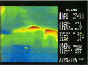 |
showing heat gain from missing knee wall insulation.
The home has 325 square feet of single glass with aluminum frames. Windows generally have insect screening on the exterior and blinds on the interior. Most of the windows are well shaded by generous 3 - 4 feet overhangs around the building's perimeter.
The home contains standard appliances. Hot water is provided by a storage-type 40 gallon electric resistance tank. The kitchen has an electric range and microwave oven with a built-in dishwasher. Food storage is provided by a 23.5 cubic foot side-by-side refrigerator with a through the door ice dispenser.
There are five ceiling fans in the home, although the owners are judicious in their use and estimate that on average only a single unit is operating at any given time. The living room has a large entertainment center with television, VCR, cable converter box and stereo. The master bedroom has a second television and stereo and the study has a computer and printer. The living room has a large salt-water aquarium with pump and lighting which are on most of the day. Lighting in the home is all incandescent except over the kitchen and in the garage. Two standing floor lamps - halogen torchieres - are the primary source for lighting in the living room.
The home has a 15,000 gallon swimming pool which is served by a 1.5 horsepower pump. The pool is unheated, but the circulation pump is generally operated for 6 hours per day in the winter and 8 hours per day during the summer season.
The building is conditioned by a 3.5-ton split system air conditioner with electric strip heat. The indoor air handler unit is located in the unconditioned garage. A programmable thermostat controls the system. The programmable thermostat sets up the interior temperature to 85oF during week day daytime hours between 8 AM and 4 PM; 83oF at 4 PM and 80oF beginning at 5:30 PM. The thermostat is set to 80oF during other hours and weekends.
The home is occupied by two working adults and a pet dog. On weekdays, both husband and wife depart the home for work at approximately 7 AM arriving home at approximately 6 PM. Both are typically home weekends. The occupants generally ventilate rather than use the air conditioner during the months of November - March. Located in South Florida, the homeowners reported very little use of the central heating system.
Monitoring
In the spring of 1995, site was fully instrumented with a multichannel
data logger (Figure 3) to both measure total electrical load as
well as to isolate each of the major end-use loads. Each of the
following were individually metered:
- Total electricity
- Air conditioner and air handler
- Hot water
- Refrigerator
- Range
- Dryer
- Washer
- Pool pump
In addition, a weather tower (Figure 4) was installed to obtain data on ambient air temperature, relative humidity and solar irradiance. We used long periods of pre and post retrofit data for each end use to determine the impact of individual measures. Changes in miscellaneous loads, including lighting and ceiling fan use, were tracked by subtracting the major electrical end uses from total. Thus, if lighting loads were altered, the differences in the estimated miscellaneous loads could be used to estimate lighting energy savings based on a pre and post retrofit monitoring protocol.

Figure 4. Weather tower being installed
Monitoring of the home in the baseline condition began on April 27th, 1995. A graphical example of 15-minute data collected from site CR1 on August 9th, 1995 is shown in Figure 5 (5a - weather data and roof temperatures; 5b - interior air data and appliance energy use; 5c - total energy use and other appliance use; 5d - water heater energy use and pool pump use.). Plots like this one, were created for each day of the monitoring project.
Figure 5a. Daily plot file for project data. Top plot is weather
data. Bottom plot measures roof and attic temperatures.
Figure 5b. Daily plot file for project data. Top plot measures
interior air temperature, relative humidity, and AC use. Bottom plot
measures refrigerator and range energy use.
Figure 5c. Daily plot file for project data. Top plate measures
total energy use and miscellaneous energy use. Bottom plot measures
washer and dryer use.
Figure 5d. Daily plot file for project data. Top plot measures
heater and hot water use. Bottom plot measures sprinkler and pool
pump energy use.
Based on the collected data over the first half year of monitoring, it was possible to characterize the magnitude of the various end-use loads as summarized in Figure 6. The pie chart shows that cooling system energy use is largest at nearly 40% of annual consumption then followed by refrigeration, dryer and hot water end-uses. Other consists of lighting and miscellaneous energy consumption.
Figure 6. Total electrical end-uses
Attic Radiant Barrier
The test home's hip roof has dark black asphalt shingles. Prior to audit, the homeowner had warned that the attic temperatures during summer were very hot. Previous test data has shown that black asphalt shingles absorb approximately 95% of incident solar radiation. Nominally, the attic floor has R-19 blown insulation although unevenly distributed.
Improving attic thermal performance is of fundamental to controlling residential cooling loads in hot climates. Accumulating research data shows that the influence of attics on space cooling demand is not only due to the change in ceiling heat flux, but often due to the conditions within the attic itself and their influence on heat gain to duct systems and on air infiltration into the building. The importance of ceiling heat flux has long been recognized, with insulation a very effective method of controlling excessive gain. However, when ducts are present in the attic, the magnitude of heat gain to the thermal distribution system under peak conditions can be often much greater than the ceiling heat flux in well-insulated attics (Parker et al., 1993; Hageman and Modera, 1996).(1)
Such heat gains can be substantially reduced in new residential housing through the use of white reflective roofing (Parker and Barkaszi, 1997). However, with an existing home with asphalt shingles, the options are more limited. Extensive research at FSEC has demonstrated the effectiveness of radiant barrier systems (RBS) in controlling attic cooling loads (Fairey et al., 1988).
On July 24, 1995, during the first summer of the monitoring, we retrofitted an RBS under the attic roof decking to reduce heat gain (Figure 7). Average maximum daily summer attic air temperatures were reduced by about 20 degrees by the installation (Figure 8). This was expected to both reduce heat transfer through the home's ceiling as well as heat gain to the attic duct system. Using days with matched meteorological conditions before and after the retrofit (Figure 9) we were able to show that peak day summer air conditioning savings were approximately 14%. Table 1 shows weekday and weekend days with sunny, but similar temperature and solar conditions pre and post retrofit.
Table
1
Matched Days Comparison for RBS Retrofit for Peak Summer Days,
1995
| Period | Date (Julian) | Avg. Amb. Temp. (oF) | Maximum
Attic
Temp. |
AC
kWh |
| Weekday
Pre-RBS Post RBS |
May 18th (138)
Aug. 8th (220) |
84.3oF
84.3oF |
138.0oF
123.0oF |
54.1
49.2 |
| Reduction | 15.0oF | 5.9 kWh (11%) | ||
| Weekend
Pre-RBS Post RBS |
June 13th (161)
Aug 7th (219) |
83.1oF
83.4oF |
135.0oF
113.3oF |
61.6
53.1 |
| Reduction | 21.7oF | 8.5 kWh (14%) |
The reductions in the attic air temperatures after the RBS installation were pronounced. The AC reduction on the hottest days in which the home is occupied (no daytime thermostat set up) was 10-15%. Savings were considerably lower on cloudy or cooler days and week day periods when the AC is run less frequently during daytime hours. Using long-term periods in the summer of 1995, before and after the installation in the radiant barrier we estimated annual air conditioning energy use was reduced by about 5.5% (~430 kWh) from the installation.(2) However, the cost of the retrofit installation was high, approximately $1,100, as compared with the $400 that might be typical with new construction. With an estimated $32 annual savings, payback appears only attractive for new construction.
Replacement of the Air Conditioning System
The greatest energy user at the study home was the eight-year old air conditioning (AC) system (Figure 10). The system was a conventional, 3.5-ton split system (York H2CC042 A06A). The air handler (York N2AHD 06A) was installed in the garage. The combination has a nominal seasonal energy efficiency ratio (SEER) of 9.0 Btu/W at rated conditions. The duct system consists of R-4 flex duct of various diameters and is located in the attic. As with many Florida air conditioning systems, the existing ducts evidenced a significant pressure drop due to long and circuitous runs and pinched segments (Figure 11).
Figure 10. Homeowner with old AC condenser unit.
Figure 11. Existing ducts showed significant pressure drop due to long, circuitous runs and pinched segments.
Average consumption during the air conditioning season (273 days of the year) averaged 28.8 kWh/day: (7,750 kWh/yr or about 37% of annual total consumption). Even though a programmable thermostat only energizes the system when the occupants are home (evenings and weekends), consumption was still quite high and the AC frequently operated without cycling. The homeowner maintained an occupied thermostat set point of only 80oF so that a low setting did not explain the elevated consumption. We extensively tested the AC unit and the duct system to isolate the source of the system's poor performance.
The duct system was suspected, but pressure tests revealed that it was relatively tight (it had been sealed as a part of FPL's duct repair program). The few leaks that were found were sealed on April 11th, 1995. With the blower door in place, we performed pressure pan tests (Figure 12) on each of the supply registers and the single return register. The highest measured pressure with respect to outdoors was 1.8 Pa - indicating that the individual duct branches are well sealed.
Figure 12. Duct pressure test.
We also used two Duct Blaster testing devices to determine the relative leakage in the return and supply sides of the duct system (Figure 13). Total CFM25 leakage of the duct system was 124; of this 59 was in the return and 65 was in the supply. Then we did a second test which isolated the duct leakage from outside the conditioned space: 63 CFM25. This indicates that much of the overall leakage is occurring around registers and boots that are leaking into the conditioned space and thus are not deleterious. We repaired one small leak in the supply which may have been 20 cfm at the operating duct pressure (~60 Pa). We suspected that much of the remaining return leakage was occurring at the air handler in the garage. Given its 1,430 square feet of conditioned area, the outside duct leakage 0.044 cfm/ft2. This compares to the 0.03 cfm/ft2 proposed as a standard for utility new homes programs. In summary, we found that the duct system of the house was well sealed and not the source of the poor cooling performance.
Figure 13. Duct leakage test.
We also used the blower door (Figure 14) to measure house tightness. The total overall building tightness was 1632 CFM50 or 7.9 ACH50. The house ELA was measured at 84.5 square inches. The results indicate a fairly tight building envelope. Estimated natural air change per hour is approximately 0.25. We noted during the blower door test that there were many large leaks in the building shell that could be seen in air moving down interior partition walls from the attic.

With the air handler operating, we measured +0.3 Pa inside with respect to outside - slight positive pressure. Most importantly, we did not measure any large negative pressure in the building which could otherwise be pulling hot air from the attic into the conditioned space.
A more complete audit of the AC air handler revealed the reason for the poor cooling performance. The indoor 3.5-ton air coil has a rated air flow requirement of 1,400 cfm. However, when measuring with a flow hood, we discovered that the return air flow was only about 550 cfm - only 40% of the recommended level. The reason was a long thirty foot length of 14- inch return flex duct which greatly increased the static pressure drop on the return side of the fan coil. The return duct was both too long and too small in diameter to accommodate the required air flow for proper system operation. We performed a test of the AC efficiency at an 83oF outdoor temperature - a typical condition since the average temperature in the month of August is 81oF.
To see how the low flow condition affected system operation, the following test data were taken:
Tsupply = 52.7o
Treturn = 79.5o
Qreturn= 550 cfm
RHreturn= 58%
RHsupply= 86%
The sensible cooling was then:
550 x 60 x (79.5 - 52.7) x 0.018 = 15,920 Btu/hr
Total cooling considers the enthalpy of the return and supply air (33 and 21 Btu/lb, respectively). There is 13.25 cubic feet of dry air per pound of dry air at the mean temperature.
Qtot = 550/13.25 x 60 x (33- 21) = 29,887 Btu
This equates to an EER of approximately 6.3 Btu/W at an 83oF outdoor temperature. Although the configuration removes a lot of moisture, it does so at great cost to the efficiency of the machine. Except for the high return air temperatures, the coil would likely ice up. A visual inspection revealed extensive mold growth on the wet evaporator coil (Figure 15).
Other
field research at additional locations, showed that low evaporator
coil air flow is both pervasive in Florida and responsible for a
significant decrease in cooling performance in both new and existing
homes (Parker et al., 1997). Clearly, low evaporator air flow was
largely responsible for the poor cooling system performance at the
site.
We also performed a Manual J calculation on the loads for the
home with a room-by-room calculation. The evaluation indicated an air
conditioner size of 1.93 tons. On this basis, we specified a 2.0 ton
machine for the AC retrofit. We then met the potential AC contractor
who noted that the existing duct sizes (14" flex) were inadequate
for the needed air flow for the current system and the return long
duct amplified the problem.
By comparing the Manual J results with available unit, agreement was reached over the proper system to install. A 26,400 Btu/hr single-speed outdoor unit (Trane TTY024A) was matched with a variable speed indoor fan coil unit (TWE040E13). The ICM fan motor in the specified unit is much more efficient (90%) than standard types. The fan speed varies with the cooling load, but uses and speed control profile which enhances coil humidity removal. A completely new plenum box and return duct section was also fabricated, sealed and tested.
The new AC system was installed in May 31, 1996 (Figure 16) with final correction of indoor unit speed settings complete by June 4th. The installed machine has a nominal SEER of 15.0 Btu/W. A short ducted return was provided from the living room ceiling in the home to reduce system friction losses. The size of the return was maximized based on the space available for the air handler (16"). FSEC personnel met with the AC contractor when the AC system was being installed to insure an airtight plenum box was constructed.
Figure 16. New AC unit.
On August 12th, 1996 a test was performed to evaluate the new machine performance as was done with the pre-retrofit system. The data were taken on a hot summer day with a measured inlet air temperature to the condenser of 96.2oF. A resistance heating test showed a fan flow of 1019 cfm at high speed with a fan power draw of only 252 W.(3) Total air handler and compressor power draw was measured at 2419 W. A temperature difference of 20.2oF was measured across the evaporator coil with 680 ml of condensate measured over a ten minute period as a check on the measured enthalpy conditions taken before and after the coil. Measured sensible cooling was 22,230 Btu/hr; measured latent cooling was 9,550 Btu/hr for a system sensible heat ratio (SHR) of 0.70. Total cooling capacity was 31,780 Btu for an EER of 13.1 Btu/W at the test conditions. The audit test revealed that the relative space cooling efficiency was increased by over 50% by the replacement unit.
Using a year of data post installation from June 5th, 1996 - June 4th of 1997, the air conditioning consumption was reduced to 4,453 kWh for a 42% reduction in cooling energy use. Figure 17 shows the measured air conditioner energy consumption over the entire two-year monitoring period. Figure 18 shows the average daily profile of the energy savings over year long pre and post retrofit periods.
Figures 19 and 20 show homeowner comfort "take-back" after the installation. This was specifically mentioned by the homeowners; once the improved system was installed they chose to lower the nighttime temperatures in the home to improve comfort. However, Figures 21 and 22 show a comparison of the daily air conditioning energy use at the home plotted against the measured temperature difference between the inside and ambient over year long periods. Both periods show the expected behavior; air conditioning rises with increasing temperature difference between the interior and exterior. The AC use in the baseline home increases by 12.2% for each degree F change in the daily temperature difference. However, the slope of the regression line between the two systems (4.89 kWh/F vs. 2.25 kWh/F) shows that the improved AC system reduced cooling system electricity consumption by 64% at equivalent loads.
With measured
annual savings of 3,259 kWh ($277/yr) against a cost of $4,071, the
retrofit has a simple payback of 15 years. This is long, but the
existing unit was near the end of its useful life. Also, the new
variable speed air handler unit measurably reduced operating sound
levels and improved interior comfort levels by reducing interior
humidity.
Solar Hot
Water System
The study home had a conventional electric resistance water heater (Ruud Pacemaker PE-40-2) with two 4,500 W elements. The measured hot water temperature from the tap was 117oF; the tank is set to 130oF at its thermostat. The tank is located in the garage (Figure 23). Both showers have a low flow showerhead rated at 2.5 gpm at maximum flow.(4) We monitored both water heater electricity use as well as hot water consumption from May 1995 - February 15, 1996 when a small solar water heating system was added.
Figure 23. Conventional electric resistance water heater showing water use meter.
Measured hot water consumption averaged 30 gallons per day - considerably less than the "typical" DOE standard profile of 64 gallons per day. This is at least partially due to the small household size - two persons with no children. Measured hot water electricity consumption averaged 3.7 kWh per day prior to installation of the solar system (1,350 kWh/yr) and closely tracked measured daily hot water consumption (Figure 24). The remaining variation in energy use shown in the scatter plot is primarily due to seasonal differences in inlet tap water temperature to the tank.
Solar water heating systems are a demonstrated technology to significantly reduce water heating energy use in Florida (Merrigan, 1983). The solar hot water heater chosen for the project is an add-on system, so called because it is added onto the existing 52-gallon hot water tank. Manufactured by Solar Development Inc., the system won the 1991 Florida Governor's competition for a low-cost solar water heating system. To lower costs, the collector is only 20 square feet (2 x 10' flat plate collector) and the unit has no parasitic energy consumption since a small solar electric photovoltaic panel powers its DC pump. The installed collector on the south facing roof-top is shown in Figure 25.
Figure 25. Solar hot water system.
Performance of the system has been very good. Since its installation and final checkout on February 16, 1996, back-up water heating electricity use has averaged 1.09 kWh/day or a savings of 72% in spite of a slight increase in hot water consumption. The change in 15-minute water heating electricity demand is shown in Figure 26. The daily hot water use and electricity demand profile before and after retrofit is shown in Figures 27 and 28. Measured annual energy savings using a year pre and post installation was 951 kWh/yr, with a value of approximately $81 at current energy prices. The solar water heater was professionally installed for $1,650 so that the simple payback is long - 20 years. However, do-it-yourself persons could easily install a kit version of the system for about a $1,000 with more attractive economics.
Pool Pump Replacement
Like many Florida homes, the study site has a 15,000 gallon pool (Figure 29). The pool plumbing uses conventional 1.5" PVC piping to provide adequate flow to an automatic pool cleaner. The homeowner operated the one horse power pool pump for seven hours per day during winter months and 10 hours per day during the rest of the year. Based on previous field research, we knew that opportunities for reducing energy existed within this end-use (Messenger and Hays, 1984).
Figure 29. View of the pool.
The measured pool pump electricity at the study home during a nine month baseline period was large: 9.3 kWh per day or 3,386 kWh/yr. We measured 37.4 total feet of head on the pool's circulation piping and calculated that a 3/4 horsepower pump would adequately provide the flow needed for the operation of the pool cleaner. The existing pool pump was an A.O. Smith C48K2PU101 with a continuously running electrical demand of approximately 1.3 kW. We then located a very efficient 3/4 hp pool pump, a Max-E-Glas PE5DL. The pump was replaced on March 25, 1996 (Figure 30).(5) Average power demand under the operating load is approximately 900 Watts. Figure 31 shows the 15-minute pool pump electrical demand over the monitoring period; Figure 32 shows the same data averaged over the daily profile.
Since retrofit, pool pump energy has averaged 6.0 kWh/day - savings of approximately 35%, or about 1,210 kWh/yr ($103). Since the cost of the new pump was $320, and contractors will install such equipment for approximately $50, the payback on such an improvement is less than four years. The automatic pool cleaner operated acceptably with the new pump; the homeowner noted no difference in its performance in the period after the installation.
Super-Efficient
Refrigerator
Replacing existing inefficient refrigerators with more efficient
models is a proven method to reduce residential energy use (Parker
and Stedman, 1992).The existing refrigerator at the site was typical
of many Florida homes: a 23.5 cubic foot General Electric TFF 24RC
side-by-side refrigerator. Manufactured in 1983, the DOE energy guide
label annual energy use for this unit was 1,748 kWh. Experience indicated
that refrigerator energy use in Florida homes is often 10-20% greater
than the label values due to the higher interior temperatures. However,
we were surprised by the consumption which averaged 8.33 kWh per
day for an annual energy use of 3,040 kWh per year!
Figure 33 shows that the energy use of the existing unit rose in the late summer of 1995 when the anti-sweat case heaters were switched on. Analysis showed that consumption prior to activation of the heaters (turning off the "Energy Miser" switch) was 7.0 kWh/day, increasing to 9.0 kWh/day with the heaters on. The 3,040 kWh used over the year (with and without the case heaters) was 15% of the annual household energy use. This also a significant addition to the level of internal heat gain.
On February 16th, 1996 a new 25 cubic foot Whirlpool ED25PS*D*O refrigerator was installed in the home (Figure 34). This Whirlpool model won a utility sponsored competition for the Super Efficient Refrigerator Program (SERP) and was procured specifically for the project. The new side-by-side refrigerator was slightly larger than the original unit, but included the same through the door features. Measured consumption after its installation over an entire year was dramatically lower, averaging just 2.32 kWh per day or an estimated 849 kWh per year. Although this is greater than the estimated energy use for the SERP refrigerator (641 kWh/year), the savings still represent a 73% reduction in energy use from the refrigerator. The consumption profile of the two refrigerators over the 24-hour cycle is shown in Figure 35. With a measured energy savings of 2,191 kWh/year against a purchase cost of $1000, annual savings are estimated at $186 with a simple payback of 5.4 years.
Figure 34. Energy-effiecient refrigerator.
Increased Attic Ventilation
Even with the installed radiant barrier system, the heat gain of the attic remained excessive. The home has small non-continuous screen soffit vents under the eaves of the roof (see Figure 36), but no ridge vents. The roof has black asphalt shingles, which get very hot; we measured surface temperatures in excess of 180oF. During baseline monitored, we recorded attic air temperatures of 143oF on the hottest days in July 1995.
The ceiling has 6 inches blown fiberglass insulation irregularly distributed over the 1,768 ft2 attic floor. The actual R-value is not probably greater than R-15 as installed. Also, missing knee wall insulation in the cathedral ceilings results in further compromise to thermal performance (see Figure 2 and Figure 3).
With the attic radiant barrier installed in July of 1995, the peak attic air temperature dropped by almost 20oF and produced measurable savings in air conditioning consumption. However, we were still displeased with the magnitude of the attic temperatures (peaks 120oF on clear summer days). To try to further reduce this load, on August 12, 1996 we had a "Cobra Ridge Vent" ridge vent added to the attic.
Approximately 60 lineal of the roof ridge was cut to provide the added vent area. A two inch wide strip was cut from the ridge apex and the mesh ridge vent was then placed over the gap. The mesh was then topped off by shingles. According to the manufacturer, the effective free vent area is 16.9 square inches per lineal foot. On this basis, the added vent area is 7.0 square feet. Observing the installation (Figures 37 and 38), we had questions regarding its potential effectiveness. However, when the installation was complete, we could detect hot air exiting the ridge vent.
In order to gauge the actual effectiveness, we performed a simple calculation based on the metered data. We compared the difference between the attic air temperature and measured ambient air temperature for one month before and after the retrofit. The result over a 24 hour profile is shown in Figure 39. The plot clearly shows that the added ridge vent reduced the attic air temperature. The average temperature difference between the attic and ambient over the daily cycle fell by 1.51oF, although the peak afternoon air temperature was lowered by 4.4oF. Assuming, 1500 square feet of conditioned attic floor area at R-19 and 375 square feet of R-4 duct, the change in the peak conductance is approximately 800 Btu/hr. With the given efficiency of the air conditioner (~13 Btu/W at peak conditions), this represents approximately a potential 60 W (2%) reduction in peak AC power. Annual energy savings from the retrofit were estimated at approximately 1% (45 kWh) based on a regression analysis of before and after cooling energy use.
Energy Use of Other Appliances
The home has an electric resistance range and as well as a clothes washer and dryer which were not retrofit during the project. However, the existing clothes dryer was changed to one with a larger capacity (and wattage) on December 5th, 1995. The larger clothes dryer increased this energy end-use by 26%.(6)
Cooling is not a large energy end-use in this household. The two adults in the household often eat out and measured range electricity consumption was fairly low relative to typical reported range energy use.(7) Measured energy use of the three appliances over a one year period averaged about five percent of total annual energy use:
Table
2
Energy Use of Household Appliances
| Appliance | kWh/Day | Annual kWh | Percent of Total |
| Range/Oven
Clothes Dryer Clothes Dryer #2 Clothes Washer |
0.84
1.60 2.01 0.14 |
307
584 732 53 |
1.5%
2.8% 3.5% 0.4% |
Figure 40 shows the measured appliance load profiles at the site over a one year period after the new dryer was installed.
Retrofit of Home Lighting
A previous study had already demonstrated the savings available from reductions to home lighting energy use (Parker and Schrum, 1996). A comprehensive lighting inventory on the house was performed as summarized in Table 3. The home contained 59 lamps under 17 controls (switches). The total connected lighting load was 3,700 W. Obviously, however, not all lighting is powered at any one time. Thus, in June of 1996, after a year long period of baseline monitoring, we substituted high efficiency compact fluorescent lamps and other high efficiency fixtures for the more frequently used lamps. The connected lighting load was reduced to 1.5 kW or by 60%.
The miscellaneous electrical loads at the site were determined by subtracting the various measured end-uses from the total load. What was left over is lighting loads, energy use from the stereo, clocks, rechargeable phone, etc.
One problem with the subtraction method of monitoring (major end uses are subtracted from total load) is that the residual loads left over include lighting as well as numerous other loads, such as the three TVs, two VCRs, home computer, electric clocks, dishwashers, vacuum cleaners etc. Consequently, in addition to the electrical metering, individual time-of-use light loggers (Pacific Science & Technology TOU-L) were deployed on each of the lighting fixtures in the home to establish actual on-time of each (Figure 41). Several of the TOU- plug loggers were also used on plug-in fixtures. The idea was to determine how the "pure" lighting loads compared with those determined by subtraction from miscellaneous loads.
Figure 41. Installed light logger on bathroom ceiling fixture.
Table
3
Household Lighting Inventory
| Switch | Area | Lamp/Fixture | Total Watts | Replacement Type |
|
1
2 |
Kitchen
Counter Lighting Overhead Lighting |
50 W Halogen (3)
F40CW T12 (4) |
150
190 |
No change
F32 T8 (2)= 78W# |
|
3
4 |
Dining
Over Table Aquarium Lamps |
50 W Halogen (3) FR40T12 I (2)* |
150
200 |
No change
F32 T8 (2)= 60W |
|
5
6 |
Living
Room
Floor Lamp Torchiere Track lighting |
475 W Halogen (1)
50 W Halogen (4) |
475
200 |
39 W CFL (2)= 78W
No change** |
|
7
8 |
Study
Floor Lamp Torchiere Ceiling fan light |
475 W Halogen (1)
60 W I (1) |
475
60 |
39 W CFL
15 W CFL |
| 9 | Hallway
Overhead flood lamps |
75 W PAR (2) | 150 | 16 W CFL (2)=32W |
| 10 | Guest
Bedroom
Ceiling fan light |
60 W I (1) | 60 | 15 W CFL (1) |
| 11 | Master
Bedroom
Wall sconces |
150 W Halogen (2) | 300 | No change |
| 12 | Bath
Vanity Lamps |
40 W I Globes (12) | 480 | 15 W CFL (4)=60W |
| 13 | Master
Bath
Vanity Lighting |
40 W I (12) | 480 | 15 W Globes (4)=60W |
|
14
24 |
Garage
General Overhead Garage Door Lamp |
F40CW T12 (4)
40 W I (2) |
190 80 |
F32 T8 (4)= 120 W
No change |
|
15
16 17 |
Outdoor
Lighting
Front Porch Back Porch Pool lighting |
25 W I Globe (1)
25 W I Globe (1) I lamp |
25
25 Unknown |
15 W CFL Globe
15 W CFL Globe No change** |
*
With Aqua Ballast 960 VLH TC-P
** Homeowner indicated these were almost never used.
#Used Octron 4100K F032/841 lamps/high output electronic ballast
Total = 59 lamps on 17 controls
Total connected load = 3690 W or 3.7 kW
After retrofit = 1467 W or 1.5 kW
The light logger monitoring began in February 1996 and extended through May of the same year. An example of the recorded data is shown in Figure 42. The plot shows the average on-time of the overhead kitchen lighting (190 Watts total). The composite load from all of the light loggers was then aggregated depending on the wattage of the lighting load on each. These loads were then used to create daily lighting load profiles for each room in the home as shown in the attached figures. The comparative data from both the "miscellaneous" load data captured by the central data logger was then compared with that recorded by the individual lighting loggers.
The homeowners use modern floor standing torchiere lamps to provide a good portion of the lighting in the home. One is used in the main living room with the other in use in the study. These lamps have become very popular due to their low expense (selling in local Home Depots for only $14.95). Although providing a very bright indirect illumination, the lamps use considerable electricity. Models vary in the electricity consumption at full output from 300 to over 400 W depending on vintage. Because of the intense heat of the halogen element, they are also a fire hazard. Underwriter's Laboratory (UL) has disapproved new models with wattage greater than 300 W.
Two
of the older vintage of these lighting fixtures are used in the
study home, estimated by the homeowner to be used at least three
hours or more each evening. Although dimming, the homeowners reported
always using each at full output. We used a digital power analyzer
to measure the electrical use of the torchieres. At full output
they each drew 475 Watts.(8) Based
on this information and the estimated load hours we calculate that
3 kWh/day is due to the halogen torchieres. Given the fact that
the homeowner indicates that both of the torchieres are typically
used in evenings, the likely demand from both is very similar to
the peak - around 900 Watts. Moreover, with both on there is a
3,000 Btu/hr sensible load on the air conditioner.
To address this energy use, we constructed three compact fluorescent
lamp (CFL) substitutes for the existing torchieres. The prototypes
were designed around the General Electric D-lamp with an electrical
demand of only 39 W (Figure 43). From photometric testing we were
able to determine that two of the CFL torchieres would provide equal
or greater light output than the single 475 W torchiere used in the
home in the living room.
Figure 43. Retrofitted Torchiere
We installed two of the prototype models on June 29th 1996. Figures 44 and 45 (bottom of this page) show the living room illuminance before retrofit with the single torchiere and afterwards with the two CFL models. Interestingly, the homeowner preferred the light from the new torchieres to the previous single model. We also changed out the kitchen lighting from a fixture with four-tube F40CW T12s with magnetic ballasts to two F32 T8s with a high output ballast and reflectors to obtain more light from the fixture (Figure 46). CFLs of various sizes and types go elsewhere with the lighting change out. The first phase of the change was done on May 30th, 1996, with the torchieres altered a month later. The last incandescent lamps were replaced on August 3rd.
 |
 |
| Figure 45. Two 39 W CFL torchieres after retrofit. |
Figure 46. David Floyd examines T8 lamps used to replace overhead kitchen lighting.
Table 4 shows both the average number of hours which each major fixture was used within the various spaces along with the fraction of the measured daily lighting energy. Results are not always proportionate - the torchieres use much more energy than the hours would seem to indicate because of their large wattage. Pre-retrofit lighting energy consumption was on the order of 2,550 kWh/year. The table also shows the estimated savings from using the product of the recorded fixture on-time from the lighting loggers times the wattage reduction. This method of estimation calculates a daily savings of 1,402 kWh - or roughly 45% of pre-retrofit consumption.
Table
4
Fraction of Daily Electric Lighting Energy used by Room and Fixtures
| Location | Daily
kWh
(Pre-retrofit) |
Avg
No.*
Hours Day |
Retrofit
W
Reduction |
Estimated
Savings
(kWh/day) |
| Outdoor
Kitchen Kitchen counter Garage Master Bedroom Study Torchiere Study fan light Guest Bedroom Dining Room Living room torchiere Guest bath Aquarium lighting Master bath Hallway |
0.32
0.49 0.09 0.02 1.29 0.52 0.03 0.02 0.05 1.20 0.19 1.68 1.01 0.05 |
6.4
2.6 0.6 0.1 4.3 1.1 0.6 0.3 0.3 2.5 0.4 8.4 2.1 0.3 |
20
112 0 70 0 436 45 45 105 397 260 140 260 118 |
0.13
0.29 0.00 0.01 0.00 0.48 0.03 0.01 0.03 0.99 0.10 1.18 0.55 0.04 |
| Total | 7.00 | 3.84 |
* Measured by light logger.
Subtracting all the major electrical end-use from total consumption at the study home, lighting and measured miscellaneous loads are large averaging 14.2 kWh/day or 5,253 kWh per year. Thus, at 25% of annual use, this is the second largest end use in the home after air conditioning (40%). The data analysis above suggests that approximately half of this amorphous end-use is made up of lighting with a peak at 9 PM of approximately 1.3 kW. This end-use also likely makes up a large portion of the internal heat gains load on the air conditioner since most of this energy use is released to the interior of the building.
Data analysis in the year before and after the lighting retrofit showed that miscellaneous energy consumption dropped from 5253 kWh to 3913 kWh - a reduction of 1340 kWh. This is very close to the estimate derived from using the light loggers.
A comparison of the miscellaneous energy use at the household before and after the lighting retrofit is shown in Figure 47. The impact of holiday related lighting each December is clearly evident in the 15-minute data. The comparative 24-hour loads profiles are shown in Figure 48. Not surprisingly, the plot shows that the lighting energy savings are concentrated during the evening hours. The lesser reduction during the morning is due to the fact that only a portion of the bathroom vanity and bedroom lighting could be retrofit.
The economics of the lighting retrofit measure looks particularly attractive. With an overall cost of approximately $400 and a savings of $115/yr, the measure has a simple payback of just under four years.
Ceiling
Fans
Ceiling fans make up another sizeable segment of household energy
use in Florida residences. Typical homes have 4- 5 ceiling fans and
there are over 30 million fans in use around the state. Previous
analysis has shown that ceiling fans can either save cooling energy
or use more energy than is saved depending on usage patterns and
thermostat set-up behavior (James et al., 1996). Typical users reported
having 2.5 fans on at any one time with the average fan operated
13.4 hours per day. We suspected, however, that the study homeowner
would use their fans much less since they are aware of the implications
of leaving ceiling fans on for long periods in unoccupied rooms.
We monitored the on-time of the five ceiling fans in the household using motor loggers. The loggers were left in place for a full year. Figure 49 showed one of the motor loggers being placed on one of the fans. Table 5 provides the measured on-times of the fans and the estimated annual energy use (kWh).

Table
5
Measure Ceiling Fan Use
| Fan Room Location | Hours Per Day | Estimated Annual kWh |
| Dining
room
Living room Study Master Bedroom Guest Bedroom |
0.3
2.1 1.1 8.6 1.2 |
4
31 16 126 18 |
| Average | 2.7 | 195 |
The data collected from the loggers showed an average fan use of 2.7 hours per day in the household, ranging from 0.3 hours for the fan in the dining area to 8.6 hours per day for the fan in the master bedroom. Assuming an average fan power draw of 40 W, this equates to approximately 200 kWh used annually to operate the household's ceiling fans. Figures 50 and 51 shows the on-time profile for the ceiling fans in the living room and master bedroom of the home.(9)
Miscellaneous Loads
Since lighting was measured at approximately 2,550 kWh per year and ceiling fans approximately 200 kWh/year, over 2,500 kWh or about 13% of total energy use is unaccounted by the measured end uses. This consumption comprises miscellaneous electricity use (Rainer et al., 1992). Typically, miscellaneous energy use consists of loads from appliances too small to otherwise consider as separate end-uses. Loss in house wiring are also unaccounted for; this may be as large as 1% of total loads.
To obtain an idea of magnitude, we metered a variety of miscellaneous equipment in the home with the digital power analyzer to assess their loads. We also used plug loggers to record the on-times of some of the devices. Results are given in Table 6.
Table
6
Measured Miscellaneous Electricity Loads in Site Home
| Item | Watts | Hours/Day | Annual kWh |
| Security
system
Portable phone #1 Portable phone #2 100 gallon aquarium pump Entertainment center - above when off Master bedroom TV - above when off Portable radio - above when off Microwave oven Microwave clock Toaster oven Espresso maker Monitor & computer Laser printer |
15.0
1.6 1.2 41.0 210.0 18.0 150.0 5.0 7.0 2.0 600.0 5.0 460.0 360.0 115.0 250.0 |
24.0
24.0 24.0 24.0 6.0 18.0 1.51* 22.5* 1.0 23.0 0.120* 23.88 0.10 0.10 1.49* 1.61* |
131
14 11 359 460 118 83 41 3 17 26 43 17 13 63 146 |
1,545 kWh or 4.2 kWh/day |
|||
* Measured directly using plug logger.
Not measured: flashlight charger, rechargeable drill, two clocks, garage door opener. This likely add up to approximately 15 W or ~130 kWh/year.
The demand of the items that are constantly on, but not in use was surprisingly large: 43 W (375 kWh/yr) or 4% of total consumption. The so called "phantom loads" from transformers, clocks and timers, which are increasingly common in U.S. households, were half of this load.(10)
Economics
The objective of the project was to explore the maximum feasible energy savings in an existing Florida residence and as such was not intended to be economic. Nevertheless, we did track the cost of the various measures installed so that relative assessment of economic performance could be performed. Table 7 lists the various measures, their costs, estimated savings and simple payback.
Table
7
Economics of Installed Measures
| Retrofit
Measure
Description |
Installed
Cost
($) |
Estimated Annual Savings kWh ($) | Simple
Payback
(Years) |
| Radiant
barrier system (RBS)
High efficiency air conditioner Solar water heater Efficient pool pump High efficiency refrigerator High efficiency lighting Attic ventilation |
$1084 $3587* $1649 $ 320 $ 999 $ 400 $ 410 |
430 ($37)
3260 ($277) 950 ($81) 1210 ($103) 2190 ($186) 1340 ($115) 45 ($4) |
29.3
12.9 20.3 3.1 5.4 3.5 113.9 |
| Total | $8449 | 9375 ($800) | 10.6 |
*includes FPL utility rebate of $484
Even though not intended as an economic demonstration, the package of installed measures have a simple payback of under 11 years corresponding to an after-tax simple rate of return on investment of about 9.5%.
Some measures were much more cost effective than others. Perhaps most interesting, options seldom considered in residential efficiency assessment - replacement of the pool pump, refrigerator and lighting - turned out to be the most cost effective. Other measures such as the addition of a radiant barrier would be much more cost effective for new housing.(11)
Conclusions
A graphic display of the changes in energy consumption over the monitoring period are shown in Figure 52. The measured reduction over the entire year was approximately 45% as shown in Figure 53. When using the utility bills in the year previous to the monitoring, the reduction was about 40% (Figure 54). In any case, the projected demonstrated the technical feasibility of reducing household energy use between 40 and 45%, depending on the basis of the reference period. The absolute energy savings were between 8,000 and 10,000 kWh/year.
Energy savings varied by end-use: savings were over 42% of space cooling and over 70% for water heating and refrigeration. Lighting energy was cut by more than 50% and pool pumping energy by 35%.
The primary intent of the project was to demonstrate maximum feasible energy reductions in existing Florida housing rather than economically justifiable levels. Nevertheless, the economics were not entirely unattractive. The cost of the overall measures was approximately $8,450. With a measured annual utility cost reduction of $680 - $880, the simple payback of the collection of improvements was approximately 11 years.
One of the most important conclusions drawn from the study was that measures seldom considered in residential energy assessments - pool pumps, lighting and refrigeration - were the most cost effective to retrofit. A large portion of the space cooling energy savings from the AC retrofit were due to cooling system evaporator air flow and the large resulting improvement to space cooling efficiency.
References
Fairey, P., Swami, M. and Beal, D., 1988. RBS Technology: Task 3 Report, FSEC-CR-211-88, Florida Solar Energy Center, Cocoa, FL.
James, P., Sonne, J., Vieira, R., Parker, D. and Anello, M., "Are Energy Savings Due to Ceiling Fans Just Hot Air? Proceedings of the 1996 Summer Study on Energy Efficiency in Buildings, American Council for an Energy Efficient Economy, Vol. 8, p. 90, Washington D.C.
Merrigan, T., 1983. Residential Conservation Demonstration: Domestic Hot Water, Final Report, FSEC-CR-90-83, Florida Solar Energy Center, Cocoa, FL.
Messenger, R., Hays, S., Duyar, S., Trivoli, G, Vincent, J, Guttmann, M., Robinson, J, Litschauer, B., Jarvis, J. and Pages, E., 1982. Maximally Cost Effective Residential Retrofit Demonstration Program, Florida Atlantic University, Boca Raton, FL.
Messenger, R. and Hays, S., 1984. Swimming Pool Circulation System Energy Efficiency Optimization Study, prepared for Florida Power and Light Company and the National Spa and Pool Institute, Florida Atlantic University, October, 1984.
Parker, D., 1990. "Monitored Residential Space Cooling Energy Consumption in a Hot-Humid Climate: Magnitude, Variation and Reduction from Retrofits," Proceedings of the 1990 Summer Study on Energy Efficiency in Buildings, Vol. 9, p. 253, American Council for an Energy Efficient Economy, Washington D.C.
Parker, D. and Schrum, L., 1996. Results from a Comprehensive Residential Lighting Retrofit, FSEC-CR-914-96, Florida Solar Energy Center, Cocoa, FL.
Parker, D., Fairey, P., Gueymard, C., McIlvaine, J. and Stedman, T., 1992. Rebuilding for Efficiency: Improving the Energy Use of Reconstructed Residences in South Florida, FSEC-CR-562-92, Florida Solar Energy Center, Cocoa, FL.
Parker, D. and Stedman, T., 1992. "Measured Electricity Savings of Refrigerator Replacement: Case Study and Analysis," Proceedings of the 1992 Summer Study on Energy Efficiency in Buildings, American Council for an Energy Efficient Economy, Vol. 3, p. 199, Washington D.C.
Parker, D., Sherwin, J, Shirey, D. and Raustad, R., 1997. "Impact of Evaporator Coil Air Flow in Residential Air Conditioning Systems," ASHRAE Transactions, Vol. 96, Pt. 1, American Society of Heating, Refrigerating and Air Conditioning Engineers, Atlanta, GA.
Rainer, L., Greenberg, S. and Meier, A., 1992. "The Miscellaneous Electricity Use in Homes," Proceedings of the 1992 Summer Study on Energy Efficiency in Buildings, American Council for an Energy Efficient Economy, Vol. 3, p. 263, Washington D.C.
Synergic
Resources Corporation, 1992. Electricity Conservation and Energy
Efficiency in Florida: Phase I Final Report, SRC Report No.
7777-R3, Synergic Resources Corporation, Bala Cynwd, PA.
1. A simple calculation illustrates this fact. The study house has a 1,500 square foot ceiling with R-19 attic insulation. Supply ducts typically comprise a combined area of ~25% of the gross floor area (see Gu et al. 1997, and Jump and Modera, 1994), but are only insulated to R-4. With the peak attic temperatures measured at 135oF, and 80oF maintained inside, a UA deltaT calculation shows a ceiling heat gain of 4,300 Btu/hr. With R-4 ducts in the attic and a 57oF air conditioner supply temperature, the heat gain to the duct system is 7,300 Btu/hr if the cooling system ran the full hour under design conditions - approaching twice the ceiling flux
2. Regression results for daily AC energy were as follows from data for the summer of 1995. Average delta T from June - September was 1.68oF
Pre RBS: AC kWh = 42.136 + 5.480 (delta T)r2 = 0.82
Post RBS: AC kWh = 40.915 + 4.923 (delta T)r2 = 0.82
3. This compares to 26% greater measured fan power for the pre-retrofit air handler (319 W) to produce half as much air flow as the replacement unit.
4. Although supposedly low flow shower heads, the measured maximum shower flow using a catch buket was 4.5 gpm as opposed to the rated 2.5 gpm.
5. Audit revealed a pump pressure of +2.5 psig on the supply side and -28.0 psig on the suction side. Based on the pump curve, this equates to a total system operating resistance of 37.4 feet of head.
6. It was possible to determine that the 26% increase in clothes dryer consumption was not due to increased dryer use. This was done by comparing clothes washer energy consumption over periods when each dryer was in use. Clothes washer energy use was about 5% greater after the purchase of the new dryer, but not nearly to the level of the increase seen from the new appliance. The reason for this increase is unexplained, but could be due either to lower drying efficiency or more complete drying of clothes. The new dryer clearly showed increased peak demand due to the larger elements in the unit.
7. Utilities report that typical range electricity use in Florida averages 630 kWh a year - about double that measured in the two person household (SRC, 1993).
8. We purchased and tested two of the least expensive new lower wattage torchieres with a three position switch: operating power was 156 W at the low position and 267 W at full output. However, power factor, although unity at full output was adversly affected - 0.70 - at the low position.
9. A sister study to the one described, used motor loggers to measure the use of ceiling fans in a home where the occupants are more typical and do not always exercise vigilant control over fan operation. In this household, the average fan use of five installed fans is 12.6 hours per day (very close to the survey average) with an estimated annual energy consumption of 920 kWh! Assuming that this is a more typical circumstance, ceiling fans may represent an average of 6% of total annual residential energy consumption (14,900 kWh) in the typical single family Florida home. Also, if only a third of the 30 million ceiling fans in the state were operating during the utility summer peak hour, they would represent an aggregate power demand of approximately 400 MW!
10. The magnitude of this miscellaneous energy use should not be underestimated. Assuming 50 Watts of "phantom loads" in the average Florida household (over six million), this would represent a constant electrical generation requirement of 300 MWe-- nearly equal to the output of a new combined cycle electric power plant.
11. The
cost of an RBS would be approximately $400 in a new home of the
size evaluated. This would reduce the simple payback to about 11
years
*
for
Florida Energy Office
2555 Shumard Oaks Blvd.
Tallahassee, FL 32399
© 2007-2014 University of Central Florida. The Florida Solar Energy Center (FSEC)
is a research institute of the
University of Central Florida.
For more information about FSEC, please contact us or learn more about us.
Find us on Facebook!