

Reference Publication: Karkaszi, S., Parker, D., "Florida Exterior Wall Insulation Field Test: Final Report," Oak Ridge National Laboratory, Oak Ridge, TN, December, 1995. Disclaimer: The views and opinions expressed in this article are solely those of the authors and are not intended to represent the views and opinions of the Florida Solar Energy Center. |
Florida
Exterior Wall Insulation Field Test:
Final Report
Stephen
Barkaszi, Jr., Danny S. Parker
Florida
Solar Energy Center (FSEC)
FSEC-CR-868-95
EXECUTIVE SUMMARYThe Florida Solar Energy Center (FSEC) and Oak Ridge National Laboratory (ORNL) have conducted a field test of exterior insulation applied to Florida masonry residences. Approximately 50% of Florida's six million existing residences are of concrete block construction. Many of these homes, particularly those 15 years or older, have uninsulated walls.
Within the project, two single-family homes in Central Florida were extensively monitored to measure the energy savings of the technology. The primary objective was to examine the effect exterior insulation has on air conditioning (AC) energy use and peak electrical demand for two typical residences. A secondary objective was to gain practical experience with the system costs and application technique.
A before/after test protocol was followed with the exterior insulation retrofit of the homes occurring in mid summer of 1994. Instrumentation was calibrated and setup at these sites in March. Electrical power use and meteorological data were collected for the spring and first half of summer while the homes were in their base configuration. Data collection continued after exterior insulation had been retrofit for the balance of the summer.
Two data analysis methods (matched days and long-term periods) and a simulation model were used to determine the savings in AC power use. The data showed good agreement between the methods for estimation of the insulation's impact on air conditioning use at both sites. The indicated summer season savings were from 9% - 14% (3 to 5 kWh/Day) of AC use at Site 1 and savings were estimated to be -1% (-1 kWh/Day) at Site 2. Peak AC reductions between 4 and 5 PM were approximately 7% (154 Wh) at Site 1 and 1% (17 Wh) at Site 2.
Analysis of individual matched days indicated that the differing savings at the two sites may be largely explained by the thermostat settings maintained inside the two homes. Site 1, which maintained an average interior temperature of 73°F realized a savings, while Site 2 with a 79°F set point did not. A fundamental conclusion of the study was that exterior wall insulation will produce savings in Florida homes only if a low cooling thermostat setting is desirable.
Simulation analysis of a prototype home was performed using the DOE-2.1D computer program. These results confirmed the important role that the gradient between interior and exterior air temperature plays in the effectiveness of insulation on exterior masonry walls in reducing cooling needs. Secondary interactions with insulation performance were seen from wall solar absorptance and house ventilation schedule.
BACKGROUND
One common construction technique for single-family residences in the Southern United States utilizes masonry (concrete block) walls with a slab foundation. Houses having block walls are typically more air-tight than those having wood-frame walls, but are often constructed with little or no wall insulation. Wall insulation retrofits are usually limited to the exterior of the house because other methods are not practical when the block cores are sealed and interior walls are finished. Insulating the perimeter slows the heat transmission rate through the wall system. An added benefit of exterior insulation is the potential use of the block's thermal capacitance to shift cooling peak demand and minimize interior air temperature fluctuations. The Florida Solar Energy Center (FSEC) and Oak Ridge National Laboratory (ORNL) have conducted a field test to monitor the change in cooling energy use associated with exterior wall insulation retrofitted to homes in Central Florida.
PREVIOUS RESEARCH
A research project in 1990 dealing with the energy performance of buildings in Saudi Arabia evaluated 14 wall system assemblies (Grondzik, 1992). Wall panels measuring 700 mm by 800 mm were installed in a south facing wall of a test building. The project compared various insulation types and placement including: interior, exterior, and mid-wall. Thermocouple temperature sensors were placed at wall assembly interfaces and heat flow meters were positioned on the interior surface.
Wall system performance was rated by the net heat flow. Expanded polystyrene (EPS) insulation (50 mm thick) placed on the exterior surface of a masonry wall reduced the heat flux by approximately 63%. Mid-wall insulation reduced the heat flow by 71% and interior insulation out-performed both by decreasing heat flow by 80%. Conclusions reported in this study are drawn from a short data collection period (three weeks) but show that wall system performance can be significantly improved through insulation in an extremely hot climate.
Cooling energy performance of homes retrofitted with wall insulation has been evaluated in hot, dry climates with mixed results. ORNL conducted a field test in 1991 to evaluate the performance of exterior wall insulation for single-family homes in Scottsdale, Arizona (Ternes and Wilkes, 1993). Eight masonry homes were retrofitted with extruded polystyrene foam and were covered with a cementitious stucco finish. This project utilized a site built method for the installation in an attempt to reduce costs and evaluate installation techniques. Costs for the retrofits ranged from $3,610 to $4,500, with an average price of $3.34/ft².
The ORNL Arizona field test measured an annual average savings of 491 kWh (9%) with savings for individual sites varying from -106 kWh/year (-3%) to 1,319 kWh/year (18%). Average peak hour AC electrical use was reduced 15%, from 4.26 kW to 3.61 kW. The peak reduction was identified as a primary benefit of the retrofit for utilities. Consumers could cost-effectively benefit from the energy savings only if the insulation was included as part of a home improvement or renovation.
A modeling study for the Arizona project (McLain, 1992) used the DOE-2.1D building simulation program and a detailed attic performance program to estimate air conditioning (AC) energy use. The model was calibrated using the Arizona field test houses and the predicted electricity consumption agreed well with metered data for five of the eight houses. The fractional savings were within good agreement for all eight homes. Average cooling energy savings for the homes in Arizona was determined to be about 12%, assuming a 78°F cooling thermostat set point. The calibrated model was run for many cities in the southern U.S. and savings of 8% to 10% were estimated. However, savings of only 1% to 4% were predicted for coastal regions, Florida in particular. The peak cooling energy reduction was found to be more consistent throughout the country, with estimated reductions ranging from 8% to 12%.
BUILDING DESCRIPTION
Two occupied single-family block homes located in East-Central Florida were selected for evaluating cooling energy savings derived from an exterior wall insulation retrofit. Both homes were constructed with uninsulated masonry walls on uninsulated concrete slabs. A split-summer pre- and post-retrofit protocol was followed to determine the effectiveness of the measure. This test method used the test houses as their own reference which was necessary due to the small sample size and also minimized the study period. Both houses were instrumented during the early Spring of 1994. 15-minute electrical consumption, house temperature, and meteorological data were collected at each site from Spring 1994 through the Fall of 1994.
Site #1
The first exterior insulation test site (EI1) was a single-family 1450 ft² one-story building located in Cocoa, FL. The appearance of the house at the start of the retrofit is shown in Figure 1. Roof construction was a low-slope built up roof with a peak running along the short axis and rafters extending to the outer walls. Roof reflectance measurements were made at the site and the average value was 21%. 3.5 inches of rock wool were installed in the attic space over the main portion of the house and 8 inch fiberglass batts were installed over part of the 285 ft² converted garage space on the west side of the house. A 135 ft² room within the converted space had neither attic insulation nor AC supply ducts, but a door to the room was open at all times during the test.
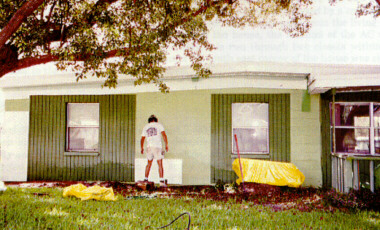
Figure 1. Appearance of test site 1 prior to the insulation
retrofit.
Initially, the unfinished exterior block walls had been painted light green. Moderate shading on the north side of the house was provided by a large tree. East and west walls had no vegetation to provide shading but were affected by fences and adjacent homes in the early morning and late afternoon hours. An estimated 35% of the south wall received direct sunlight with the remaining 65% having been completely shaded by a 21 ft by 10 ft porch roof.
Air conditioning was provided by a Rudd UPGA split system heat pump with an EER of 9.52 and a COP of 3.25 @47oF. The condensing unit was located on the south side of the house east of the screened porch. The air handler was located in a hall closet with louvered doors just outside of the main living area. Duct-work to the bedrooms and bathrooms was run through the attic space and the remaining supply ducts were within the conditioned space. There was no return duct and the return grill and filter were at the bottom of the indoor unit. The duct-work was tested, repaired, and sealed as part of other work conducted in 1992. A sketch of the floor plan and AC system layout was given Appendix A of the interim report.
Site #2
The second exterior insulation site (EI2) was a single-family 1800 ft² single-story home located in Merritt Island, FL. Roof construction is conventional trusses with gable ends and shingles covering the plywood decking. A white ceramic coating having a recently measured albedo of approximately 0.5 was applied to the roof surface in 1991 for reducing solar gains through the roof system. The attic was well insulated with approximately two inches of fiberglass covered by an additional six inches of blown cellulose yielding an nominal thermal resistance of 25 ft²·h·oF/Btu. Air infiltration from the attic area into the conditioned interior had been largely eliminated by a previous audit and retrofit at this site.
Outside block walls were covered with a thin layer of stucco and painted white prior to the retrofit at this site. The north wall was extensively shaded by a carport at the west end and trees at the east end. The east wall was partially shaded by low vegetation and an adjacent home. A 24 by 10 foot porch on the south shades approximately 40% of the wall and another 20% was shaded by shrubs. There was no vegetation shading the west wall but the neighboring house was approximately 20 feet away and blocked a portion of the late afternoon solar irradiance.
A Bard PH1130 heat pump was used for air conditioning at this site. The rated EER was 9.92 and the COP was 3.10 @ 47oF for this packaged unit which had been installed in May of 1994. Flexible, insulated supply ducts were run through the attic space. There are two return locations, one at the east end of the living area which is partially obstructed by a cabinet and a second at the west end of the bedroom hallway. The return duct-work from the living area return is run through the attic to the west side of the house, the location of the AC unit. Approximately 12 feet of duct for the main return is run through two closets within the conditioned space. The utility room supply vent in the south east corner of the house was closed off, but a door to the kitchen was typically open.
RETROFIT PROCEDURE
A commercially available exterior insulation and finish system (EIFS) was chosen for testing and evaluation instead of the site-built method described by Ternes et al. (1993) because of the popularity and availability of the commercial systems. Sto Industries' residential R-wall System was selected for use at both sites in this study. The system used EPS rigid foam boards, fiberglass mesh reinforcement in the exterior base coat, and a 100% acrylic finish.
The wall insulation retrofit was performed by a local contractor specializing in EIFS work. The installation procedure began by pressure washing the exterior surfaces to remove any dirt or loose paint. Sheets of 1.5 inch EPS foam (R=5.8 ft2hoF/Btu) were adhered directly to the wall using a Portland cement mixture. The foam was then rasped and sanded to plane the surface so that the finish would have a uniform appearance. A base coat of mastic with embedded fiberglass mesh was applied to the foam and was allowed to dry for approximately 24 hours. The pigmented acrylic finish coat was troweled over the base coat to a uniform thickness of approximately 1/16 inch. A swirled finish texture was achieved by a second pass with a clean trowel in a circular motion. Figures 2 and 3 show the retrofit in progress and then completed at Site 1. Figures 4 and 5 show the same stages for Site 2.
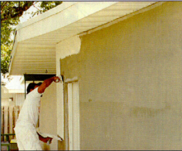
Figure 2. Acrylic polymer finish being applied at test site
#1.
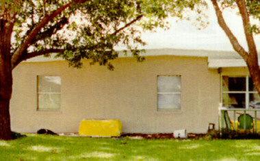
Figure 3. Appearance of the completed exterior insulation retrofit
at site #1.

Figure 4. Planing the EPS foam surface at site #2.
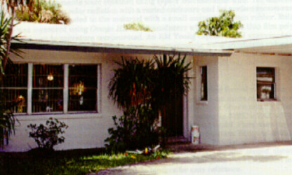
Figure 5. Appearance of the completed retrofit at site #2.
A crew of two required approximately seven working days to complete each installation. The average cost of the retrofits using this commercially available system was approximately $6,800 per home (~$3.90/ft2) which included site preparation, insulation system materials, colorfast acrylic stucco, and labor.
MONITORING PROTOCOL
The before-and-after protocol followed during this field test was similar to that used for previous research. Sites were selected based upon criteria set in the experimental design (uninsulated block walls, single family residence, etc). Retrofits were performed at mid- summer in an attempt to provide like weather conditions in the pre- and post- periods. Work began at Site #1 on July 20 and was completed on August 1, 1994. The Site #2 retrofit began August 2 and was finished on August 11. The split-summer procedure has drawbacks in that independent meteorological variables must be matched for the two intervals if the comparison is to be valid. Effort was made to ensure that insolation, ambient temperature, interior temperature, and occupant life style were similar for both data collection periods. Control over meteorological conditions is limited to selecting the appropriate time for the retrofit based on historical peaks. Thermostats were maintained at an occupant determined setting for the duration of the project to provide a consistent interior temperature. It was requested that homeowners not make any major changes to their homes (remodeling, additions, etc) during the test period to minimize changes in occupant behavior.
Audit
Each of the home audits follow a survey protocol provided by ORNL. The purpose of the audit procedure was to identify the physical characteristics of the structure and energy consumption devices in order to evaluate the efficiency of the building. Also characterized by the audit were the occupant energy use preferences and schedules. Completed audit forms were provided in the interim report.
Instrumentation and Data Collection
Instrumentation was installed in the homes to measure the various parameters used in determining the energy savings potential of an EIFS system. Meteorological conditions monitored at the sites were: ambient air temperature, solar irradiance, wind speed, and relative humidity. Interior conditions monitored included wall system temperatures, roof system temperatures, interior air temperature and relative humidity. Interior and exterior wall system temperatures were obtained in order to help characterize changes brought about by the insulation. Temperatures were collected in different rooms based on anecdotal reports from ORNL's monitoring of the Arizona homes which indicated changed thermal performance in interior zones due to the addition of exterior insulation. Table 1 shown on the next page lists the parameters measured and the associated units.
The total house, air conditioner and major appliance electrical uses were monitored using watt-hour transducers. Measured air conditioner energy use was fundamental to the project objective. However, a number of additional electrical measurements were taken in order to isolate electrical end-uses taking place within the conditioned interior of the home. Since the level of internal gains can have a dramatic impact on cooling needs, multiple points of electrical energy use within each house were directly measured to provide an improved match between the pre- and post- conditions. This also required isolation of electrical loads occurring outside the home.
Temperature measurements were obtained using type-T thermocouple wire. The ambient air sensor was shielded from solar radiation with a vented enclosure and for surface measurements the thermocouple was bonded to the material with a small amount of silicon rubber. Relative humidity was measured using Omega HX-92V transducers which utilized a thin film polymer capacitor and was temperature compensated. An RM Young cupped wheel anemometer was positioned above the roof line for wind velocity measurements. Solar irradiance values were obtained via a Li-Cor pyranometer utilizing a silicon photodiode sensor. Electrical power use was measured using Ohio Semitronics WL41RX series 120 and 240 volt watt-hour transducers with split core current transformers.
Analog and pulse outputs from the sensors were converted to digital format and stored using a Campbell Scientific model CR10 datalogger. Sensor measurements are made at 0.2 Hz and are averaged over 15 minute intervals. Electrical power was totalized over fifteen minute intervals. Data were transferred from the dataloggers via telephone modem to FSEC's VAX 4000 on a nightly basis. Once processed and archived, data for each site were plotted. Plots were inspected each morning to ensure reliable data collection and proper sensor function. Samples of the daily data for site 1 on July 11, 1994 are presented in Figures 6 and 7. The first plot page shows the meteorological, wall and roof system, and interior conditions, and the second shows the electrical power use for the various monitored end-uses (7a, 7b, 7c). Similar plots were generated for site 2 and the plots for both sites were compiled in binders for easy reference.
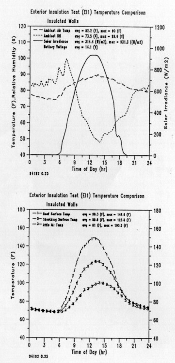
Figure 6a. Sample plot of interior and exterior conditions at Site 1 on July 11, 1994.
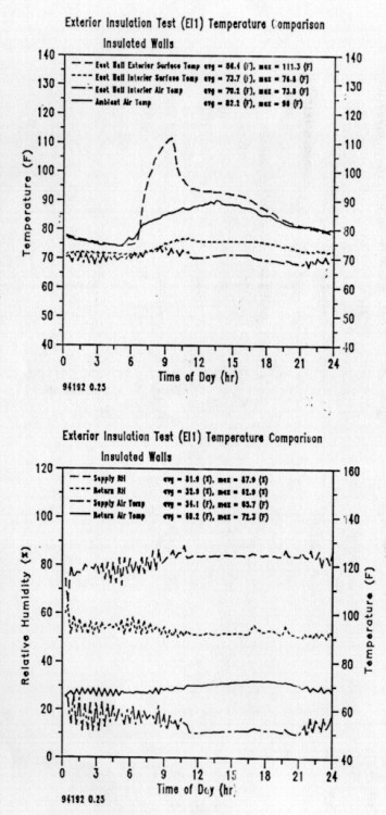
Figure 6b. Sample plot of interior and exterior conditions at Site 1 on July 11, 1994.
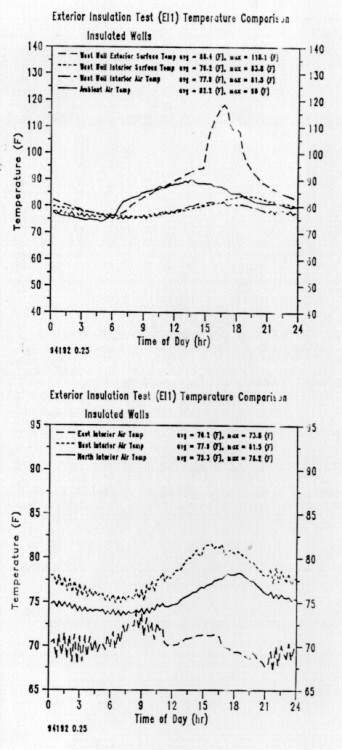
Figure 6c. Sample plot of interior and exterior conditions at Site 1 on July 11, 1994.
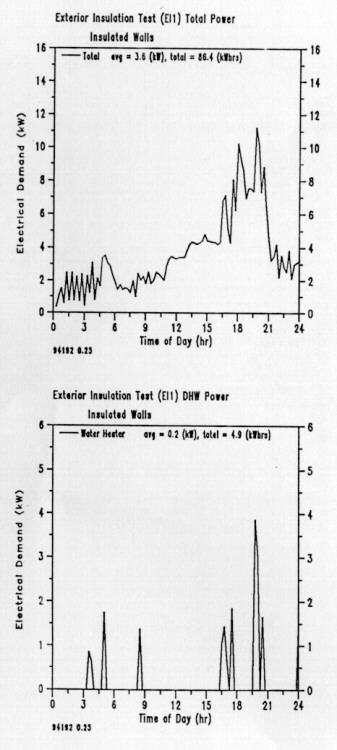
Figure 7a. Sample plot of measured power use at Site 1 on July 11, 1994. Top plot is total power and bottom plot is water heater power.
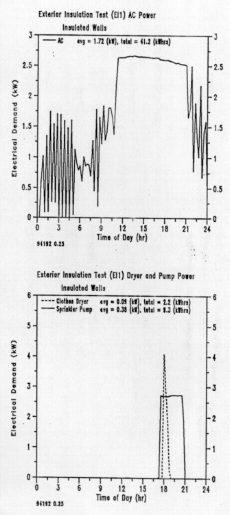
Figure 7b. Sample plot of measured power use at Site 1 on July 11, 1994. Top plot is AC power and bottom plot is clothes dryer and sprinkler pump.
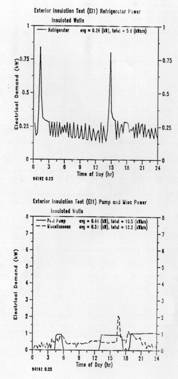
Figure 7c. Sample plot of measured power use at Site 1 on July 11, 1994. Top plot is refrigerator power and bottom plot is pool pump and miscellaneous power use.
Table
1
Exterior Insulation Field Test Measurement Parameters
| Ambient
air temperature Solar irradiance Wind speed Relative humidity |
oF W/m2 m/s % |
| West
exterior wall surface temperature' West interior wall surface temperature' West room interior air temperature' East exterior wall surface temperature' East interior wall surface temperature' East room interior air temperature' Roof surface temperature1 Sheathing underside temperature1 Attic air temperature' Living area temperature' Living area relative humidity' AC supply air temperature' AC supply relative humidity' AC return air temperature' AC return relative humidity' |
oF oF oF oF oF oF oF oF oF oF oF oF oF oF oF |
| Total
house Air conditioner condenser Refrigerator Water heater Clothes dryer Pool pump1 Irrigation pump1 Freezer2 |
Wh Wh Wh Wh Wh Wh Wh Wh |
1 EI1 site only. 2 EI2 site only.
DATA ANALYSIS
Two analysis methods and a simulation model were employed in determining the effect of the exterior wall insulation on air conditioning use at the two sites. A matched days comparison method estimated savings using individually paired days with similar weather conditions from the pre- and post-retrofit periods. Analysis of "composite days" utilized long-term averages of continuous data segments before and after the treatment.
Matched Days
A matched days analysis was used to investigate the change in energy use after the retrofit by identifying single days with similar conditions from the pre- and post- data sets. Comparable days must be within minimum parameter tolerances established for daily averages of: ambient temperature (+1oF), solar irradiance (+20 W/m²), internal temperature (+1oF), and interior appliance electrical use (+80 Wh). Having identified matching days, savings were computed from the averaged AC power use. All of the parameters were pooled together and a daily composite average was obtained. Tables 2 and 3 summarize the results of this analysis for the two sites. The matched days method estimates a 8.9% savings (3.2 kWh/day) in cooling energy use for Site 1 and a 5.5% AC use increase (1.4 kWh/day) at Site 2.
Table
2
Matched Days Comparison for EI1
| Exterior Insulation Test EI1 Matched Days Average | ||||||
| 19 Matching Days Identified | ||||||
| Amb Temp (oF) | Solar Irr (W/m²) | Int Temp (oF) | App. Use Avg. kWh/day | AC Use Avg. kWh/day | SAVINGS (%) | |
| Before | 81.8 | 265.9 | 73.4 | 13.4 | 36.0 |
8.9 |
| After | 81.9 | 261.6 | 73.5 | 13.2 | 32.8 | |
Table
3
Matched Days Comparison for EI2
| Exterior Insulation Test EI2 Matched Days Average | ||||||
| 44 Matching Days Identified | ||||||
| Amb Temp (oF) | Solar Irr (W/m²) | Int Temp (oF) | App. Use Avg. kWh/day | AC Use Avg. kWh/day | SAVINGS (%) | |
| Before | 80.9 | 239.6 | 79.0 | 10.3 | 26.4 |
-5.5 |
| After | 81.0 | 240.2 | 79.0 | 10.4 | 27.8 | |
Long-Term Periods
Composite days were created for each data collection period by averaging the data from a series of days. This method differs from the matched days analysis because averages are computed for each hour from the successive days. Long-term periods could then be viewed as a single representative day. Selection of the days was done such that the number of readings averaged would be maximized and the variation in the independent parameters would be minimized. Averages and standard deviations of the daily averages for the various parameters and the estimated savings for the two sites are given in Tables 4 and 5. The standard deviations show that the variation in daily averages was comparable for the pre- and post-retrofit periods. Figures 8 and 9 are plots of the hourly composite averages for the site conditions, interior temperatures, and cooling energy demand for test sites 1 and 2.
Table
4
Long-Term Periods Comparison for EI1
| EI1 | Julian Days | Amb temp (°F) | Solar Irr (W/m2) | Int Temp (°F) | App. Use (kWh/day) | AC Use (kWh/day) | Savings (%) | |
| Before | Average | 160 - 192 | 80.7 | 235.3 | 73.8 | 15.7 | 31.7 | 14.5 |
| Std. Dev. | 2.4 | 62.1 | 1.6 | 4.3 | 9 | |||
| After | Average | 214 - 246 | 80 | 212 | 73.2 | 12.8 | 27.1 | |
| Std. Dev. | 2 | 71.4 | 1.5 | 4 | 9.6 | |||
Table
5
Long-Term Periods Comparison for EI2
| EI2 | Julian Days | Amb temp (°F) | Solar Irr (W/m2) | Int Temp (°F) | App. Use (kWh/day) | AC Use (kWh/day) | Savings (%) | |
| Before | Average | 167 - 188 | 81.4 | 234 | 79.2 | 9 | 26.1 | -4.9 |
| Std. Dev. | 2 | 56.1 | 0.4 | 3.4 | 5.5 | |||
| After | Average | 239 - 260 | 81 | 208.3 | 79.1 | 12.1 | 27.4 | |
| Std. Dev. | 2.4 | 58.5 | 0.3 | 3.5 | 6.3 | |||
Figure 8. Composite day comparison of site conditions
and AC demand at EI1.
Figure 9. Composite day comparison of site conditions and cooling energy use at test site 2.
Average Peak Reduction
Peak reductions in electrical use for cooling were obtained from the composite days analysis. Values for the reduction in power use for the time periods from 4 to 5 PM and 5 to 6 PM (EDT) were calculated. Hourly power use and the associated savings for the before and after periods are listed in Table 6. Peak reduction as described above was for a composite day of hot, mild, and warm days; not the absolute peak for the season or year. Reduction of power use for a typical day during peak hours is significant to Florida's power generation facilities because of the high occurrence of periods of operation at capacity.
Table
6
Average Peak Reduction for EI1
| Period | Average Electrical Use | Average Reduction in Use | ||
| Pre-retrofit | Post-retrofit | |||
| 4 - 5 PM | 2130 Wh | 1976 Wh | 154 Wh | 7.2% |
| 5 - 6 PM | 2150 Wh | 1844 Wh | 306 Wh | 14.2% |
Table
7
Average Peak Reduction for EI2
| Period | Average Electrical Use | Average Reduction in Use | ||
| Pre-retrofit | Post-retrofit | |||
| 4 - 5 PM | 1825 Wh | 1808 Wh | 17 Wh | 0.9% |
| 5 - 6 PM | 1956 Wh | 1984 Wh | -28 Wh | -1.4% |
Measured Changes to Wall and Room Thermal Conditions
A composite day analysis was also utilized to determine changes in wall system performance and to compare interior room air temperatures before and after the insulation retrofit. After the retrofit, interior wall surface temperatures were expected to decrease while an increase in the exterior wall surface temperatures were anticipated due to the greater resistance to heat flow through the wall. It was estimated that the interior room air temperatures would be unchanged since the thermostat setting was unaltered. These simplistic assumptions were found to be consistent with the averaged data in most cases.
Figure 10 graphically depicts the aggregate changes in meteorological conditions, interior room air temperatures, and wall system temperatures during pre- and post-retrofit periods at Site 1. Exterior wall surface temperatures peak at significantly higher levels during the post- period. It can also be seen that the heat is dissipated more rapidly from the wall exterior and minimum temperatures are below those observed prior to the retrofit. This was especially true for the west wall where heat had been retained in the exposed block wall throughout the evening and night hours. Insulating the walls smoothed diurnal fluctuations in interior surface temperatures and lowered the peak. The interior surface was cooler in the pre- period for a short time during the average night but only by a fraction of a degree for both the East and West walls. An unexpected change at Site 1 was that interior air temperatures for the East and West rooms were found to be higher on average after the walls were insulated.
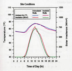
Figure 10. Composite day comparison of changes to interior room
air and wall system temperatures before and after the retrofit at EI1.
A possible explanation for the increase in interior air temperature for the East and West rooms is that the reduction in AC use decreased circulation though the house. Figure 8 indicates that the average temperature actually decreased near the thermostat, which is located on an interior wall near the center of the house. Since the house was not designed for central air conditioning, placement of the ductwork and supply vents was by convenience. Also, the West room was an addition to the house and does not have a dedicated supply vent, it relies on circulation from adjacent rooms. With the core of the house remaining cooler after the retrofit, the air conditioner would cycle longer or would not run continuously as long. This produced longer periods of stagnation and the extreme rooms of the house would warm.
A graphical comparison of the meteorological, room air temperatures, and wall system temperatures for Site 2 over the defined aggregate periods is presented in Figure 11. Averaged wall system temperature patterns were similar to those observed at Site 1. Interior surface temperatures fluctuated to a lesser degree while peak and average temperatures were significantly lower after insulating the walls. Opposite to Site 1 but consistent with expectations, average room air temperatures were reduced at Site 2 during the post-retrofit period. Usage of the AC system did not decrease at site 2, and the AC system had a return at each end of the house and dedicated supply vents for each room providing adequate circulation. One unexpected observation was a shift in the peak East exterior surface temperature from morning to afternoon. The thermocouple was field tested and did not appear to be faulty. A plausible explanation was that the wall was receiving more shade after the retrofit in the early morning due to changes sun position and vegetation growth.
Figure 11. Composite day comparison of interior room air and
wall system temperatures before and after the exterior insulation retrofit
at EI2.
The average interior air temperature at Site 2 was consistent for the two intervals as seen in Figure 9. Figure 11 shows that the greatest reduction in interior air temperature coincides with the largest decrease in interior surface temperature. This indicates that the wall load for these two rooms was lessened as a result of the exterior insulation retrofit.
Simulation Analysis
A modeling study was performed in conjunction with the field test to verify trends observed in the data collected during the exterior insulation field project. The DOE 2.1D building simulation program (LBL 1989) was used to predict cooling and heating energy use for a 1,000 square foot base building with a typical layout (see Table 5).
A parametric analysis using the following variables was performed to determine the effect on wall insulation performance: insulation type, cooling set point, natural ventilation option, and wall absorptance. A summary of the simulation assumptions is given in Table 8. Particulars for the simulated building configurations for selected runs are given in Table 9.
Table
8
Specifications for Base Building
| Primary Characteristics | |
| Building Type | Single-story, rectangular floor plan |
| Construction | Slab-on-grade, masonry walls |
| Orientation | Major axis runs East-West |
| Floor Area | 1,000 ft² (30 ft x 50 ft) |
| Roof | Asphalt shingles, plywood sheathing |
| Overhang | Full perimeter 2 ft |
| Ceiling Insulation | R-11 ft²hF/Btu |
| Roof Absorptance | 80%, 22.6 roof slope |
| Window Area | 248 ft² |
| Window Type | Single pane, shading coefficient = 0.6 |
| Heating and Cooling Equipment | |
| Heating | Electric resistance, 40,000 Btu/h |
| Cooling | 3 Ton AC, EER = 6.8, SHR = 0.75 |
Table
9
Variable Parameters for Selected Building Configurations
| Run | Set Point | Ventilation | Wall Solar Absorptance (%) | |
| Heating (oF) | Cooling (oF) | |||
| 1 | 69 | 70 | no | 0.3 |
| 2 | 69 | 70 | no | 0.4 |
| 3 | 69 | 70 | no | 0.5 |
| 4 | 69 | 70 | no | 0.6 |
| 5 | 69 | 80 | no | 0.3 |
| 6 | 69 | 80 | no | 0.4 |
| 7 | 69 | 80 | no | 0.5 |
| 8 | 69 | 80 | no | 0.6 |
| 9 | 69 | 70 | yes | 0.3 |
| 10 | 69 | 70 | yes | 0.4 |
| 11 | 69 | 70 | yes | 0.5 |
| 12 | 69 | 70 | yes | 0.6 |
| 13 | 69 | 80 | yes | 0.3 |
| 14 | 69 | 80 | yes | 0.4 |
| 15 | 69 | 80 | yes | 0.5 |
| 16 | 69 | 80 | yes | 0.6 |
Monthly cooling and heating energy use throughout the year was estimated for the above sets of parameters, each with three wall configurations: exterior insulation, interior insulation, and no insulation.
Values for annual heating and cooling energy use in each of the configurations are given in Table 10. The analysis showed that insulated walls provided a maximum cooling energy savings of 4.3% when the interior temperature was 70°F and ventilation was provided. With the higher cooling set point and non - ventilated configurations, the additional insulation provided little benefit and often produced increased energy use. Generally, the exterior insulation performed better than interior insulation in the simulations.
A significant reduction in heating energy use (approximately 1000 kWh) was produced by the addition of insulation to the simulated home in all cases. Exterior insulation out-performed interior insulation by approximately 100 kWh for each configuration. Although the interior set point was the same for each run, interactions between the heating and cooling schedules caused slight variations in the energy use.
Table
10
Annual Heating and Cooling Energy Use for Selected Building
Configurations
| Run | Heating (kWh) | Cooling (kWh) | ||||
| Insulation Type | Insulation Type | |||||
| Exterior | Interior | None | Exterior | Interior | None | |
| 1 | 578 | 726 | 1722 | 8998 | 8986 | 8890 |
| 2 | 566 | 715 | 1681 | 9027 | 9020 | 8983 |
| 3 | 556 | 703 | 1642 | 9062 | 9053 | 9071 |
| 4 | 546 | 693 | 1603 | 9092 | 9085 | 9164 |
| 5 | 510 | 677 | 1670 | 2755 | 2934 | 2471 |
| 6 | 499 | 666 | 1626 | 2792 | 2965 | 2556 |
| 7 | 490 | 655 | 1585 | 2827 | 3001 | 2641 |
| 8 | 479 | 645 | 1547 | 2858 | 3037 | 2726 |
| 9 | 733 | 836 | 1829 | 8035 | 8117 | 8221 |
| 10 | 720 | 824 | 1793 | 8060 | 8141 | 8305 |
| 11 | 707 | 812 | 1755 | 8088 | 8169 | 8381 |
| 12 | 695 | 802 | 1721 | 8111 | 8193 | 8459 |
| 13 | 710 | 823 | 1818 | 1967 | 2289 | 1932 |
| 14 | 698 | 812 | 1782 | 1987 | 2304 | 1984 |
| 15 | 687 | 800 | 1744 | 2000 | 2318 | 2043 |
| 16 | 676 | 789 | 1711 | 2014 | 2334 | 2097 |
DISCUSSION
OF RESULTS
A summary of the empirical data analysis results (Table 11) indicates that there is agreement and consistency between the methods. This indicates that the savings realized at EI1 and the increased cooling energy use at EI2 are properly described for the respective test periods. The two homes were of similar construction and experienced similar weather conditions but opposite results were produced with the introduction of exterior insulation. Major differences between the sites were the efficiencies of the cooling equipment and the interior temperatures maintained.
Table 11
Summary of Empirical Analysis Results
| Matched Days | Composite Days | ||||
| Measured AC Use | Savings | Measured AC Use | Savings | ||
| EI1 | before | 36.0 kWh | 8.9% | 31.7 kWh | 14.5% |
| after | 32.8kWh | 27.1 kWh | |||
| EI2 | before | 26.4 kWh | -5.5% | 26.1 kWh | -4.9% |
| after | 27.8 kWh | 27.4 kWh | |||
The analysis presented here do not separate week days from weekend days or account for variations in temperature and electrical use throughout the day. The weekdays and weekend days were not segregated for the analysis for the following reasons: 1) interior temperatures were constant throughout the testing period, 2) the thermostat control remained on at all times during the cooling season to provide comparable day-to-day conditions, and 3) appliance use, being a fair indicator of occupancy, was incorporated into all three analysis methods.
Simulation analysis of a prototype home similar to the test homes in this study provides an approximated estimate of expected performance. This exercise also permitted varying parameters to isolate effects. It was determined that thermostat setting, wall solar absorptance, and house ventilation strategy would be the parameters to most significantly interact with the wall insulation. In the simulation of the home configured similarly to that of EI1, having a cooling set point of 70oF and wall absorptance of 50%, the exterior insulation provided modest 3.5% annual cooling energy (293 kWh) savings.
Consistent with measured data, an increase in cooling energy use was predicted for a home similar to EI2 receiving exterior insulation. Annual cooling energy use was predicted to increase by 1.8% (35 kWh). In this case the cooling set point was 80oF and the wall absorptance was 30%. It is important to note, however, that both buildings were predicted to experience energy savings when both annual heating and cooling budgets were included. Table 12 presents a summary of the results obtained from the simulation. Appendix A provides the graphic results from the simulation cases.
Table
12
Simulation Results for Cases Similar to Monitored Homes (EI1 and
EI2)
| Cooling Set point (oF) | Absorptance (%) | Heating Energy Use (kWh) | Cooling Energy Use (kWh) | Savings (%) | |||
| pre- | post- | pre- | post- | ||||
| Case 1 | 70 | 50 | 1755 | 707 | 8381 | 8088 | 3.5 |
| Case 2 | 80 | 30 | 1818 | 710 | 1932 | 1967 | -1.8 |
While the simulated building was not a detailed description of either test home, it did provide a basis for relative comparisons. Values for energy use could not be directly related to the monitored buildings; however, general trends in performance of a configuration were apparent. A fundamental conclusion of the modeling study was that application of exterior insulation over masonry walls in Florida's climate only has a potential to significantly reduce cooling needs if a low thermostat setting is desired.
SUMMARY
Exterior insulation was retrofit onto two residential homes in Central Florida in the summer of 1994. The houses were instrumented with electrical power use data and meteorological data being collected for the first half of summer while the homes were in their base configuration. Data collection continued for the balance of the summer after the exterior insulation had been retrofit.
Use of three different methods (matched days, long-term periods, and a simulation model) to analyze the data showed good agreement on the insulation's impact on air conditioning use at the two sites. The indicated summer season savings ranging from 9% to 14% of AC use at Site 1 with a negative savings of about -5% at Site 2. Average reductions in cooling energy use during peak periods were modest at test site 1 and negligible at test site 2.
Analysis of individual matched days indicated that the differing savings at the two sites may be largely explained by the different thermostat settings maintained inside the two homes. Site 1, which maintained an average interior temperature of approximately 73oF, realized a savings, while Site 2 with a 79.0oF set point did not. DOE-2 simulation analysis of a prototype home confirmed the important role that the gradient between interior and exterior air temperature played in the effectiveness of insulation on exterior masonry walls in reducing cooling needs. Appreciable reduction to AC use in Florida homes will most likely be realized only in cases with low cooling thermostat settings. While aesthetically pleasing to the homeowners, the low energy savings clearly makes such an improvement non-cost effective from an energy-efficiency standpoint.
FUTURE WORK
Future analysis may include a more extensive investigation into time of day variation in the load profiles, possibly on a 15-minute or hourly basis. Higher resolution analysis would allow a better description of the true reduction in peak demand. Future experiments may examine load shifting potential in the exterior insulated masonry buildings. This type of testing would use an automated thermostat with pre-cooling of the structure during morning hours to shift maximum AC loads away from the utility peak in late afternoon.
REFERENCES
ASHRAE, 1989. ASHRAE Handbook - 1989 Fundamentals, American Society of Heating, Refrigeration, and Air Conditioning Engineers, Atlanta, GA.
Grondzik, W.T., 1992., Summer Performance of Fourteen Wall Assemblies in a Hot-Arid Climate, Proceedings of the 17th National Passive Solar Conference, American Solar Energy Society, Boulder, CO.
LBL, 1989., DOE-2 Reference Manual, version 2.1a, Report LBL-8706, Rev2. DOE-2 supplement, version 2.1D. Report LBL-8706, Rev 5 Supplement, Berkeley, CA: Lawrence Berkeley Laboratory.
McLain, H.A., Modeling Study of the Cooling Season Performance of Exterior Wall Insulation, Thermal Performance of the Exterior Envelopes of Buildings V: Proceedings of the ASHRAE/DOE/BTECC Conference, pp 655-667, American Society of Heating, Refrigeration, and Air Conditioning Engineers, Atlanta, GA, December 1992. Ternes, M.P. and Wilkes, K.E., Air-Conditioning Electricity Savings and Demand Reduction From Exterior Masonry Wall Insulation Applied to Arizona Residences, ASHRAE Transactions 1993, Vol.99, Part 2, pp.843-854.
Ternes,
M.P, Wilkes, K.E., and McLain, H.A., Cooling Energy Performance
and Installation of a Retrofitted Exterior Insulation and Finish
System on Masonry Residences in the Southwestern United States,
Development, Use, and Performance of Exterior Insulation and Finish
Systems (EIFS), ASTM STP 1187, M.F. Williams, R.G. Lampo, and R.G.
Reitter, II Eds., American Society for Testing and Materials, Philadelphia,
1993.
Submitted to
Oak
Ridge National Laboratory
PO Box 2008
Oak Ridge, TN 37831-6070
© 2007-2014 University of Central Florida. The Florida Solar Energy Center (FSEC)
is a research institute of the
University of Central Florida.
For more information about FSEC, please contact us or learn more about us.
Find us on Facebook!