

Reference Publication: Fuehrlein, B., S. Chandra, D. Beal, D. Parker, and R. Vieira, "Evaluation of EnergyGauge® USA, A Residential Energy Design Software, Against Monitored Data." Proceedings of ACEEE 2000 Summer Study, pp 2.115 - 2.126, American Council for an Energy Efficient Economy, Washington, DC, August 2000. Disclaimer: The views and opinions expressed in this article are solely those of the authors and are not intended to represent the views and opinions of the Florida Solar Energy Center. |
Evaluation
of EnergyGauge® USA, A Residential Energy
Design Software, Against Monitored Data
Brian
S. Fuehrlein, Subrato
Chandra, David Beal,
Danny
S. Parker, and Robin
K. Vieira
Florida
Solar Energy Center (FSEC)
FSEC-CR-1670-00
ABSTRACT
A new software, EnergyGauge USA®, is being developed for calculation of energy use in residential buildings. A simplified user interface allows buildings to be quickly defined and evaluated. Utilization of the DOE-2.1E energy simulation engine brings the computing power of hourly simulation to designers and raters. The software has enhancements to better simulate duct systems, air infiltration, attic and foundation thermal performance, heat pump part load characteristics and internal moisture capacitance.
A recurring question with building energy software, regardless of the calculation rigor, is the relative accuracy of the estimates, particularly for cooling loads. To address this question, the software was used to estimate the hourly air conditioning electrical demand in three homes extensively monitored in Apopka, Florida. Each of the homes were unoccupied, and were identical in layout and orientation, yet contained different efficiency measures. A conventional concrete block home served as the project control house while a second had better insulated walls (autoclaved aerated concrete) and double-glazed windows. The third home, constructed with wood frame walls, had solar-control windows and an attic radiant barrier.
Building geometry, construction and features were entered into the software with measured values being used for critical inputs. Monitored meteorological data was used to create weather files for the simulation and measured interior temperatures were input for each building. The resulting hourly simulation predictions for air conditioning power were then compared to the monitored values for September 1998. Analysis showed excellent correspondence between the simulated and actual data. Average error was less than 4 percent for average hourly and less than 6 percent for peak hour air conditioning usage. Maximum errors were about 10 percent.
Introduction
A new software, EnergyGauge USA®, is being developed for calculation of energy use in residential buildings. A simplified user interface allows buildings to be quickly defined and evaluated. Utilization of the DOE-2.1E energy simulation engine brings the computing power of hourly simulation to designers and raters. The software has enhancements to better simulate duct systems, air infiltration, attic and foundation thermal performance, heat pump part load characteristics and internal moisture capacitance.
A recurring question with building energy software, regardless of the calculation rigor, is the relative accuracy of the estimates, particularly for cooling loads. To address this question, the software was used to estimate the hourly air conditioning electrical demand in three homes extensively monitored in Apopka, Florida.
The Entry Level Homes
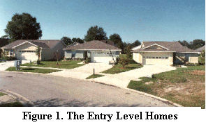 In
August 1998 three side-by-side homes were completed near Orlando,
FL (Figure 1). All homes have identical floor plans of 1187
square feet (Figure 2), similar roof and wall colors, air handler
in conditioned space, and all homes face east. The first house,
the Block house, was a base case home constructed of conventional
concrete block. Its only modification was an upgraded AC unit
(20% better than minimum code). The second home, built from
autoclaved aerated concrete (AAC), demonstrated excellent indoor
air quality (IAQ). The third house was the energy-efficient
home, built from 2x4 wood frame walls. Table 1 summarizes the
details of the three homes. In
August 1998 three side-by-side homes were completed near Orlando,
FL (Figure 1). All homes have identical floor plans of 1187
square feet (Figure 2), similar roof and wall colors, air handler
in conditioned space, and all homes face east. The first house,
the Block house, was a base case home constructed of conventional
concrete block. Its only modification was an upgraded AC unit
(20% better than minimum code). The second home, built from
autoclaved aerated concrete (AAC), demonstrated excellent indoor
air quality (IAQ). The third house was the energy-efficient
home, built from 2x4 wood frame walls. Table 1 summarizes the
details of the three homes. |
In the AAC home a 4" diameter duct delivers fresh outside air to the home through the return air plenum whenever the air handling system operates. The FanRecyclerTM is a control device that turned on the air handler fan periodically, even when there was no need for heating or cooling. Coupling this with the outside air duct ensured fresh air ventilation in the home throughout the year. The other homes rely on cracks and crevices or open windows for ventilation. The installed radiant barrier in the Frame house was a paper backed aluminum foil stapled to underside of the roof deck and inside of the roof gable ends. The homes were completed in August 1998 and monitored under unoccupied conditions between August 29 and September 29, 1998. During this month air conditioning energy use, inside, outside and attic temperatures, relative humidities and solar radiation were monitored. The home and duct air tightness and ventilation rates were measured. In addition, volatile organic compound (VOC) and formaldehyde levels were tested to compare the IAQ of the homes (Chandra et. al., 1999).
|
 |
EnergyGauge USA
Figure 3 shows the EnergyGauge USA software. This software is PC based and uses the DOE-2.1E simulation engine to allow users to examine many different energy options based on the power of hourly simulation. The hourly-based simulation allows the user to input different thermostat settings, hour by hour, to analyze their impact on the peak cooling loads. For example, changing the thermostat to 72 from 78 degrees from 8 a.m. until 5 p.m. can create excessive cooling loads during peak summer months and the new simulation would be able to predict this, hour by hour. Also, since inside temperatures can be predicted, the software allows designers to examine how design features influence comfort conditions. Another feature, as the name would imply, allows homes to be modeled in 213 cities across the US. Typical Meteorological Year data is available for all 213 cities.
Figure
3. EnergyGauge USA
Other unique features of the new software are highlighted below:
-
Simulate the interaction of duct air distribution systems and their locations (attic, crawlspace, basement, etc)
-
Evaluation of light colored building surfaces on annual cooling and heating performance and impacts on duct systems
-
Assessment of various ventilation approaches
-
Characterization of appliance and lighting loads and interaction with heating and cooling
-
Estimation and modeling of the dependence of ceiling insulation conductivity on the temperature difference across the insulation (Parker, et.al., 1999).
Defining the Inputs
All input variables must be input carefully as the accuracy of the simulation depends on the accuracy of the inputs. Table 1 shows the important inputs. The details of the walls, windows, floors, roofs and garages were taken from the blueprints and verified with on-site measurements. The lots were surveyed to determine all surrounding buildings and trees. The infiltrations were measured by the tracer gas decay method (SF6) using a photo-acoustic analyzer. The mechanical ventilation was input as zero for all three homes even though the AAC home has the FanRecycler. The FanRecycler only comsumes energy by turning on the fan even when there is no need for cooling. Since this study took place during September the FanRecycler did not add to the energy consumption of the AAC home.
Since these homes were unoccupied, the thermostat settings were under FSEC control. Figure 4 shows the hourly internal temperatures of the three homes during the monitoring period. Three different thermostat settings were seen. August 29 through September 9 (hours 1-310) was the first setting, September 10 through September 17 (hours 311-580) was the second setting and September 18 through September 28 (hours >581) was the third setting. The thermostat settings that were input are shown in Table 2:
Figure 4. Indoor Hourly Average Temperatures, by Period
Period
1 |
Period
2 |
Period
3 |
|
| Block House | 78
F |
71.5
F |
72
F |
| Frame House | 79
F |
73.5
F |
72.5
F |
| AAC House | 78
F |
72
F |
71.5
F |
Table 2. Thermostat Settings
Ambient temperatures and solar radiation were monitored and entered into the simulation. Typical Meteorological Year (TMY2) weather files were used as defaults and then modified as necessary. For detailed information on all simulation inputs as well as a step-by-step explanation of modifying the weather data please see Fuehrlein, 1999.
Results
This experiment served as a comprehensive test of the EnergyGauge USA software. The variables in this experiment were the following: 1. Three different home constructions representing base case, energy efficient and improved IAQ homes. 2. Three different periods of thermostat settings that were input into the software. These variables were tested in three periods for each house. Period one represented a warm thermostat setting and periods two and three represented a cooler thermostat setting. By testing a total of nine periods these variables were isolated.
Since many variables are being controlled, if the outputs (i.e. predicted hourly a/c energy use) of the simulation match closely with the measured data, for all three homes, for all three periods, the simulation can be considered valid for entry-level homes. Other conclusions can be drawn depending on which parts of the simulation do not match the measured data.
Figure 5. Block House, Period 1
Figure 6. AAC House, Period 1
Figure 7. Frame House, Period 1
Figures 5 through 7 show the hourly and daily energy consumption of the three houses for period one. There was an excellent relationship between the simulated and the predicted values. There was, however, an anomaly near hour 140 on day six. The measured energy consumption was very high for several hours for all three homes. This was the day that FSEC researchers performed the SF6 test on the homes. When performing the SF6 test the air handlers were on for the duration of the test. This was what caused the sharp increase in energy consumption during those few hours. This was something that the simulation would not and should not predict. These bad data points was ignored during the data analysis section. Also, the AAC house was missing data for several days during this period. This data was also ignored.
Figure 8. Block House, Period 2
Figure 9. AAC House, Period 2
Figure 10. Frame House, Period 2
Figures 8 through 10 show the hourly energy consumption for the three houses for period two. The thermostats for the houses were set near 78 degrees the last day of period one and near 72 degrees for the first day of period two. For the first day of the colder setting the air conditioner not only has to meet the steady state cooling loads but also the load from cooling down the thermal mass of the house itself. In the simulation, the warm up period has to be the same thermostat setting as the period of interest. There is no way to accurately simulate a sudden thermostat change to 72 degrees from 78 degrees. This is the reason that the measured energy consumption was more than the simulated energy consumption. The first day of data from period two was not included in the data analysis.
Figure 11. Block House, Period 3
Figure 12. AAC House, Period 3
Figure 13. Frame House, Period 3
Figures 11 through 13 show the energy consumption of the three houses for period three. Since the thermostat change was very small for all three homes between period two and three, the warm-up period will be ignored. There were no other anomalies with the data throughout period three.
Period averages were looked at in an effort to draw initial conclusions about the difference between the predicted data and the measured data. Period averages for the overall simulation, for each house, for the high thermostat and for the low thermostat settings are presented in Table 3. Table 4 shows the period averages broken down individually for each house. All units are in kWh.
Overall |
Block |
Frame |
AAC |
High
Therm |
Low
Therm |
|
| Predicted | 0.69 |
0.75 |
0.55 |
0.79 |
0.51 |
0.80 |
| Measured | 0.69 |
0.75 |
0.57 |
0.76 |
0.51 |
0.79 |
| % Error | 0.00 |
0.00 |
-3.51 |
3.96 |
0.00 |
1.27 |
Table 3. Overall Period Averages
The overall averages were practically the same showing a strong overall accuracy of the software. Isolating each building technique and thermostat setting as variables, the period average error did not exceed four percent.
Period
1 |
Period
2 |
Period
3 |
|||||||
Block |
Frame |
AAC |
Block |
Frame |
AAC |
Block |
Frame |
AAC |
|
| Predicted | 0.57 |
0.40 |
0.57 |
0.87 |
0.61 |
0.87 |
0.86 |
0.67 |
0.89 |
| Measured | 0.57 |
0.41 |
0.58 |
0.96 |
0.64 |
0.86 |
0.81 |
0.69 |
0.84 |
| % Error | 0.00 |
-2.44 |
-1.72 |
-8.42 |
-4.69 |
1.16 |
4.94 |
-2.99 |
5.95 |
Table 4. Individual Period Averages
Table
4 shows a detailed look at all nine sets of data. The high thermostat
setting represents period one for all three houses and the low
thermostat setting represents periods two and three for all three
houses. Again, regardless of thermostat setting, the simulation
model is very accurate with error never exceeding nine percent.
A second analysis was conducted to test the simulation accuracy during
peak cooling load periods. In the summertime in Florida, peak cooling
occurs between the hours of four and six p.m. Data points for the
four o'clock and five o'clock hours were isolated from the data sets
and then the error between the measured and predicted data was calculated.
Similar to Table 4 above, the data is broken down by period and by
construction technique so all nine data sets are presented.
Period
1 |
Period
2 |
Period
3 |
|||||||
Block |
Frame |
AAC |
Block |
Frame |
AAC |
Block |
Frame |
AAC |
|
| Predicted | 0.82 |
0.65 |
0.83 |
1.20 |
0.87 |
1.19 |
1.11 |
0.88 |
1.15 |
| Measured | 0.82 |
0.64 |
0.81 |
1.36 |
0.91 |
1.22 |
1.08 |
0.89 |
1.09 |
| % Error | 0.00 |
1.56 |
2.47 |
-11.76 |
-4.40 |
-2.46 |
2.78 |
-1.12 |
5.50 |
Table 5. Peak Load Error
Table 5 shows that even under extreme cooling load conditions the EnergyGauge USA software is accurate. The error only exceeded ten percent once and all other times was consistently below six percent.
Conclusions
Overall, the EnergyGauge USA software was accurate in predicting energy consumption in entry level homes. Period average errors were consistently under nine percent. Even under extreme cooling loads, i.e., in Florida, in September, between four and six p.m., the software was still consistently within six percent of the measured values, only once having an error greater than ten percent (11.76%).
Future Research
This research did not address homes other than small, entry level homes. The results of this research do not indicate an increase in error with an increase in energy consumption so there is no reason to believe that the software would not be just as accurate with larger homes. A similar study should be carried out for larger homes. This study was conducted under unoccupied conditions. In order to verify the accuracy of the software under occupied conditions, further studies must be conducted.
Acknowledgements
The homes were constructed by the Viking Builders (Mr. Paul Mashburn, president) in partnership with the Affordable Housing Institute (Mr. William T. Nolan, president). This research was sponsored by the U.S. Department of Energy, Office of Building Technology, State and Community Programs - - Mr. George James, program manager. Dr. Lixing Gu of the Florida Solar Energy Center was instrumental in modifying the TMY2 weather data file to incorporate measured data. Their support is gratefully acknowledged.
LIST OF REFERENCES
Chandra, S., Beal, D., and Fuehrlein, B., "The Entry Level Homes Project - A Case Study", Proceedings of The 8th International Conference on Management of Technology, Cairo, Egypt, March 1999.
Fuehrlein, B., "Measured and Predicted Energy Consumption in Entry Level Homes", Undergraduate Honors Thesis, University of Central Florida, Orlando, FL, 1999.
Gu, L., Cummings, J.E., Swami, M.V., Fairey, P.W., and Awwad, S, "Comparison of Duct System Computer Models to the Thermal Distribution System Test Method of Test (SPC152P)", FSEC-CR-929-96, Appendix G-4 - G-6. Florida Solar Energy Center, Cocoa, FL, November 1996.
Parker, D.S., Broman P.A., Grant, J.B., Gu, L., Anello, M.T., and Viera, R.K., "EnergyGauge USA: A Residential Building Energy Simulation Design Tool", Proceedings of Building Simulation '99, Kyoto, Japan, September 13-15th. Texas A&M University, College Station, TX, 1999.
© 2007-2014 University of Central Florida. The Florida Solar Energy Center (FSEC)
is a research institute of the
University of Central Florida.
For more information about FSEC, please contact us or learn more about us.
Find us on Facebook!